Chapter 9 Statistical Analysis
Packages needed:
 * None!
9.1 Introduction
Howdy wrangler. Now that our Tauntan datasets have been cleaned up and merged, let’s explore how to conduct a few commonly used statistical tests in R. This is R’s main strength and those of you that get hooked on R will be running all your statistical analyses in R before you know it!
In your position as the Tauntaun biologist, you will need to analyze several types of data, including both categorical and continuous data. We can’t guess at what statistical analysis you will run, but the strategy for running a statistical analysis is generally the same regardless of your approach:
- Identify the function needed.
- Read the help page.
- Execute the examples in the help page with the
examplefunction. - Use the
strfunction on the sample output so that you can determine what sort of object the analysis returns. This is crucial for prying information out of the returned object (pulling the result out of the shoebox).
Here, we will cover four commonly used statistical tests to get you going: chi-squared, t-test, correlation, and regression, and will introduce you to a process for extracting the results you need.
All of the analyses in this exercise require that your updated Tauntaun dataset is loaded into R. Let’s do that now. Remember that we are using our “super-cleaned, merged, etc” data, which is stored as an .RDS file.
Make sure to look for this in your Global Environment.
9.2 Chi-Squared Test
Our first test, chi-squared test, is a simple test best used when your research question involves categorical data (with any number of categories). This test, for example, lets you formally test whether Tauntaun fur length (short, medium, long) and fur color (grey, white) are related (or dependent) on each other. That means, generally speaking, that the likelihood of a particular fur color of a Tauntaun depends on what its fur length is; or conversely, that the likelihood of a particular fur length depends on what the fur color is.
We’ll get into the guts of the chi-square test in a bit, but let’s first remind ourselves of the structure of both the fur length and fur color fields. Use the good old str function to examine the data you want to use for your statistical test.
## Factor w/ 3 levels "Short","Medium",..: 3 3 2 2 3 1 3 1 2 3 ...## Factor w/ 2 levels "White","Gray": 1 2 1 2 1 2 2 2 2 2 ...Oh yeah, fur length and color are factors. Fur is an ordered factor comprised of three levels: short, medium, and long; the color field contains two levels: white and gray. In the background, R stores factors as integers that identify the different levels.
Now, look at the help file and arguments for a chi-squared test before we delve in further:
## function (x, y = NULL, correct = TRUE, p = rep(1/length(x), length(x)),
##     rescale.p = FALSE, simulate.p.value = FALSE, B = 2000)
## NULL
Here, we see seven possible arguments, only one of which does not have a default value. Can you find it? Yup, the argument called x must be provided and has no default. The argument called x is the column of numeric data to be analyzed, and it can be a factor. But x can also be a matrix. The argument called y is a second variable of numeric data, but you don’t need this if x is a matrix. The entries of x and y must be non-negative integers because the data are counts (frequencies) of observations within each factor, and you can’t have a negative frequency.
Let’s pause here to read the Details section in thechisq.test helpfile:
“If x is a matrix with one row or column, or if x is a vector and y is not given, then a goodness-of-fit test is performed (x is treated as a one-dimensional contingency table). The entries of x must be non-negative integers. In this case, the hypothesis tested is whether the population probabilities equal those in p, or are all equal if p is not given. If x is a matrix with at least two rows and columns, it is taken as a two-dimensional contingency table: the entries of x must be non-negative integers. Otherwise, x and y must be vectors or factors of the same length; cases with missing values are removed, the objects are coerced to factors, and the contingency table is computed from these. Then Pearson’s chi-squared test is performed of the null hypothesis that the joint distribution of the cell counts in a 2-dimensional contingency table is the product of the row and column marginals.”
It may be tempting to blow off helpfiles, but this should drive home the point that you really need to read them. If we want to do a chi-squared test on fur only, then x is a vector containing fur types, and R will conduct a goodness-of-fit test where the hypothesis tested is whether the population probabilities equal something you specify in the p argument, or are all equal if p is not given.
If instead x is a table of fur and color types, then R assumes that this a two-dimensional contingency table, and will return the Pearson’s chi-squared test (sometimes called a test for independence). This second example (a two-way contingency table) is what we are interested in here.
Let’s look at one of the examples from the chisq.test helpfile. In the example we’ll soon run, we’re going to create a dataset called M that has three columns (labeled “Democrat”, “Independent”, and “Republican” and two rows, labeled “M” and “F”). The data are all integers (positive, whole numbers), and will look something like box a below. The table in box a shows the raw data; the other tables walk you through the calculations involved in the test.
Figure 9.1: Chi Square test of independence.
This primer is not intended to be a statistical primer, but we think it will be helpful to briefly review the general approach behind statistical hypothesis testing, using the Chi-Square test as an example.
The top box (a) is our dataset. You can see that there are 239 independent females, and a grand total of 2757 voters. The margins, in red, simply sum the totals by either row or column. For example, there are 1557 total males, and 1246 total democrats. These are called ‘marginal’ values because they summarize the data by row or column in the margins. In box b, the proportion of individuals in each category are calculated as the cell value divided by the grand total. For example, 18% (or 0.18) of the voters are female democrats (484/2757 = 0.18). Once again, our marginals are calculated as the sum across a row or column. Thus, 56% (0.56) of the voters are males. Box b, then, is a simple summary of proportions given in box a.
Now, the purpose of the chi-squared test is to determine if gender and party are INDEPENDENT of each other. If they are independent, then the chance a voter is a female republican should be the probability that a voter is republican (0.34) times the probability that a voter is a female (0.44), which is 0.15. This product is called a joint probability, and box c provides the joint probabilities for all parties and genders. Check our math by hand for a few of the cells.
The final box just multiplies the joint probabilities by the grand total (2757) . . . this gives the expected number of party/gender combinations IF party and gender are independent. This is what is meant by “the null hypothesis that the joint distribution of the cell counts in a 2-dimensional contingency table is the product of the row and column marginals” in the chisq.test helpfile. If two variables are NOT independent, then if we know what party a voter is associated with, we can’t predict their sex based on the marginals . . . the two variables are dependent on one another.
The chi-squared test of independence will compare the observed numbers in box a (our data) with the numbers in box d (which is the predicted number of voters if the gender and party are independent), and generate a “chi-squared test statistic”. To get the test statistic, for each of the 6 cells we take the observed number minus the expected number, square it, and divide by the expected number. For example, looking at male democrats, the chi-squared value would be (762-703.67)2/703.67 = 4.83. Summing across all 6 cells, the final chi-squared test statistic is 30.1 (which is rounded).
Now what? Well, we need to find where this value (30.1) falls on a theoretical chi-squared distribution. The result will tell us how probable it is to observe this value (30.1) by chance alone. However, we can’t just look at any old theoretical chi-square distribution. For our voter problem, we need to use a chi-square distribution that has two degrees of freedom. Which distribution to use depends on your dataset. In our case, we are testing political party (3 levels) and gender (2 levels). Degrees of freedom is determined as the number of levels in each factor minus one, multiplied together. So in our case we have (3-1)(2-1) = 2, which means we should use a Chi-squared distribution with 2 degrees of freedom.
Let’s look at what wikipedia has to say about the theoretical chi-squared:
“In probability theory and statistics, the chi-squared distribution with k degrees of freedom is the distribution of a sum of the squares of k independent standard normal random variables.”
Hoo boy. Without going too much into the weeds, a standard normal random variable (also called a z score) is a value that is drawn at random from a distribution whose mean is 0 and whose standard deviation is one. Such a distribution is called a “standard normal distribution”, and it looks like this:
# create a vector of scores that range from -4 to +4
z <- seq(from = -4, to = 4, by = 0.1)

# get the probability of each z element with the dnorm function
y <-  dnorm(z, mean = 0, sd = 1)

# plot the standard normal distribution
plot(x = z, y, type = "l", lwd = 2, col = "red")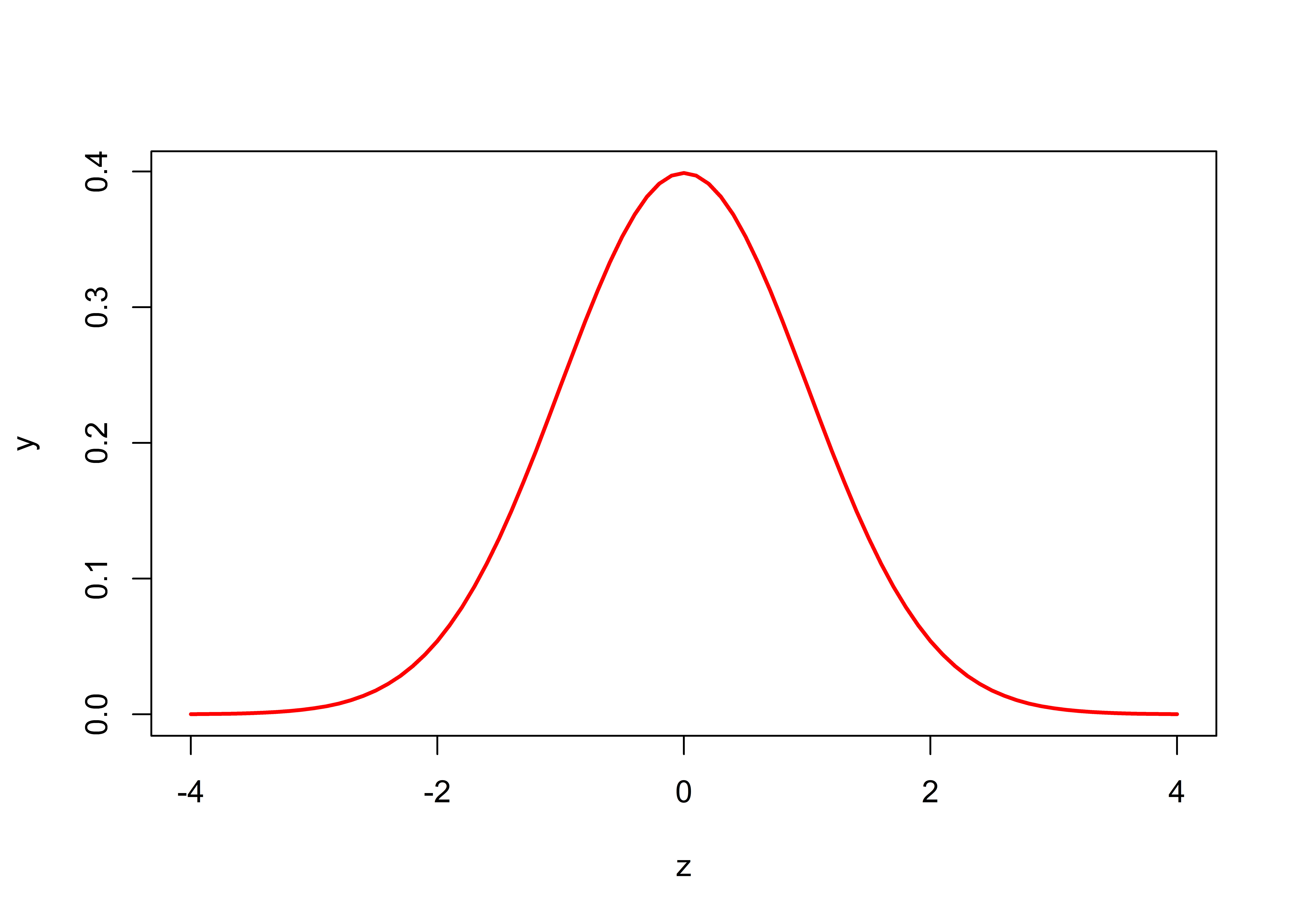
On the x-axis, we list the possible z scores that can be drawn. If we drew samples from this distribution, can you see that most values will be around 0, but a few will hover around -2 or +2, and a very, very few will hover around +4 or -4?
We can pull “values”, or z scores, out of this distribution at random with the rnorm function. Let’s pull out 10 for demonstration purposes:
## [1] 0.4945029 -0.8986097 -0.7752661 -0.2179509 -0.5712290 -0.4830192 1.1662708 -0.8561151 0.3327780 0.2286476Each time you run this function, you will generate new random numbers. (Run it again and prove this to yourself.)
Returning to our Wikipedia helpfile, “the chi-squared distribution with k degrees of freedom is the distribution of a sum of the squares of k independent standard normal random variables.” So, if we want to create a chi-squared distribution with 1 degree of freedom, we need to grab a z value from the standard normal distribution, square it, repeat this a very large number of times (say, 10,000), and then create a frequency distribution. Let’s do that now. In the code below, we use the hist function to display the frequency of squared z scores:
# generate 10000 z scores
z.scores1  <- rnorm(n = 10000, mean = 0, sd = 1)

# square the z scores
sq.z.scores1  <- z.scores1 * z.scores1

# generate a chi-squared distribution with 1 df as the frequency of the squared z scores
hist(sq.z.scores1,
     breaks = seq(from = 0, to = 30, by = 0.1),
     xlab = "X = Squared Z Scores",
     main = "Chi-Squared Distribution with 1 DF",
     freq = TRUE)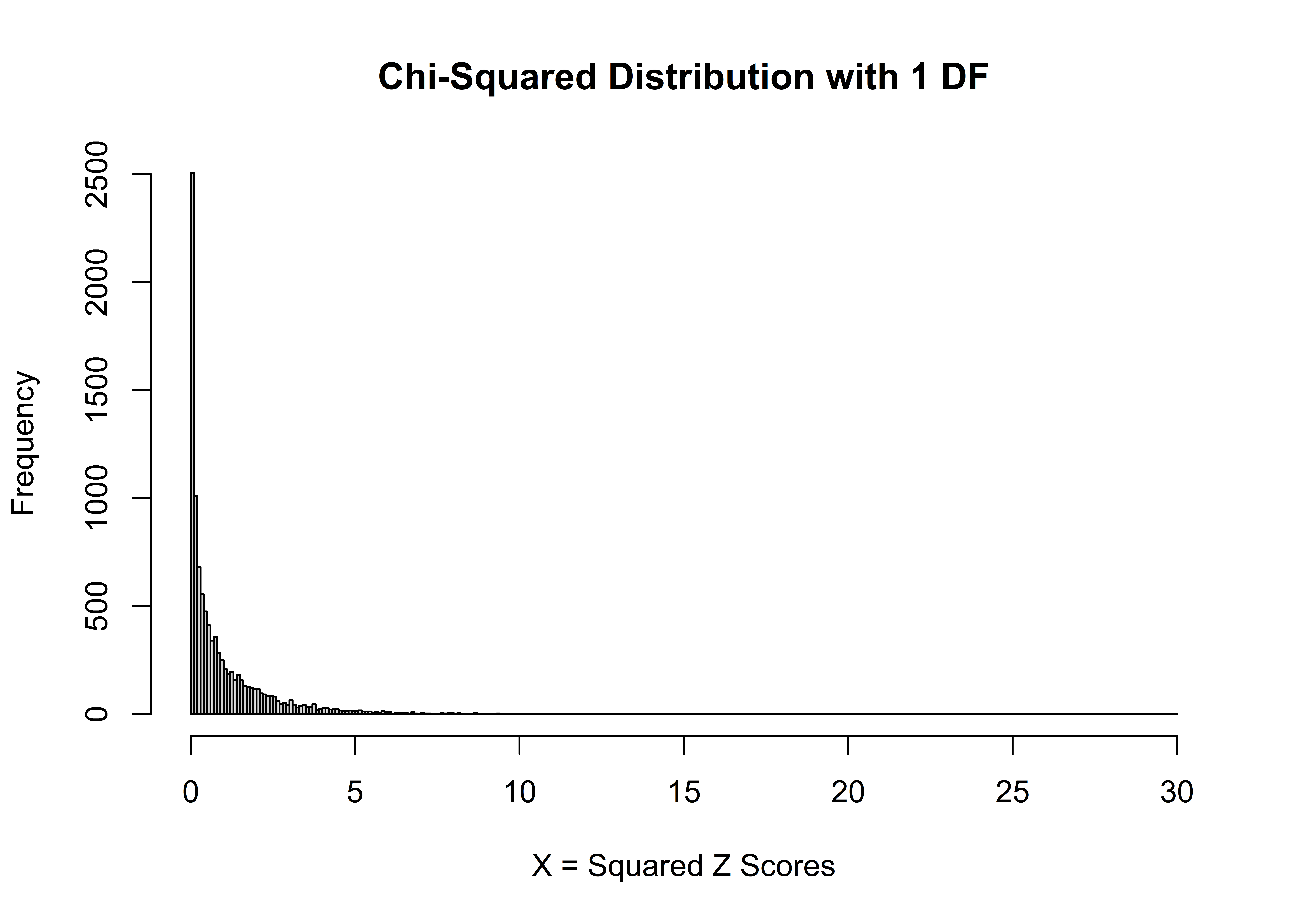
This is a “home-made” distribution of a chi-squared distribution with 1 degree of freedom. The x axis gives the squared z scores, and the y axis gives the “frequency” associated with each z score. The frequency is provided because we set the freq argument to TRUE. If freq was set to FALSE, the y-axis would read ‘density’ – this argument just scales everything so that the sum of the bars in the plot is 1.0. Notice how there is a pile of squared z scores around 0 . . . that’s because 0 is the most common z score, and 0 squared equals 0.
If we want to make a “home-made” chi-squared distribution with 2 degrees of freedom, we need to create two sets of squared z scores, and add them together:
# generate 10000 z scores
z.scores1  <- rnorm(n = 10000, mean = 0, sd = 1)

# square the z scores
sq.z.scores1  <- z.scores1 * z.scores1

# generate a second set of 10000 z scores
z.scores2  <- rnorm(n = 10000, mean = 0, sd = 1)

# square the second set of z scores
sq.z.scores2  <- z.scores2 * z.scores2

# add the first set of squared z scores with the second set of squared z scores
sum.sq.z.scores  <- sq.z.scores1 + sq.z.scores2

# generate a chi-squared distribution with 2 df as the frequency of the squared z scores
hist(sum.sq.z.scores,
     breaks = seq(from = 0, to = 30, by = 0.1),
     xlab = "x = Sum of Squared Z scores",
     main = "Chi-Squared Distribution with 2 DF",
     freq = TRUE)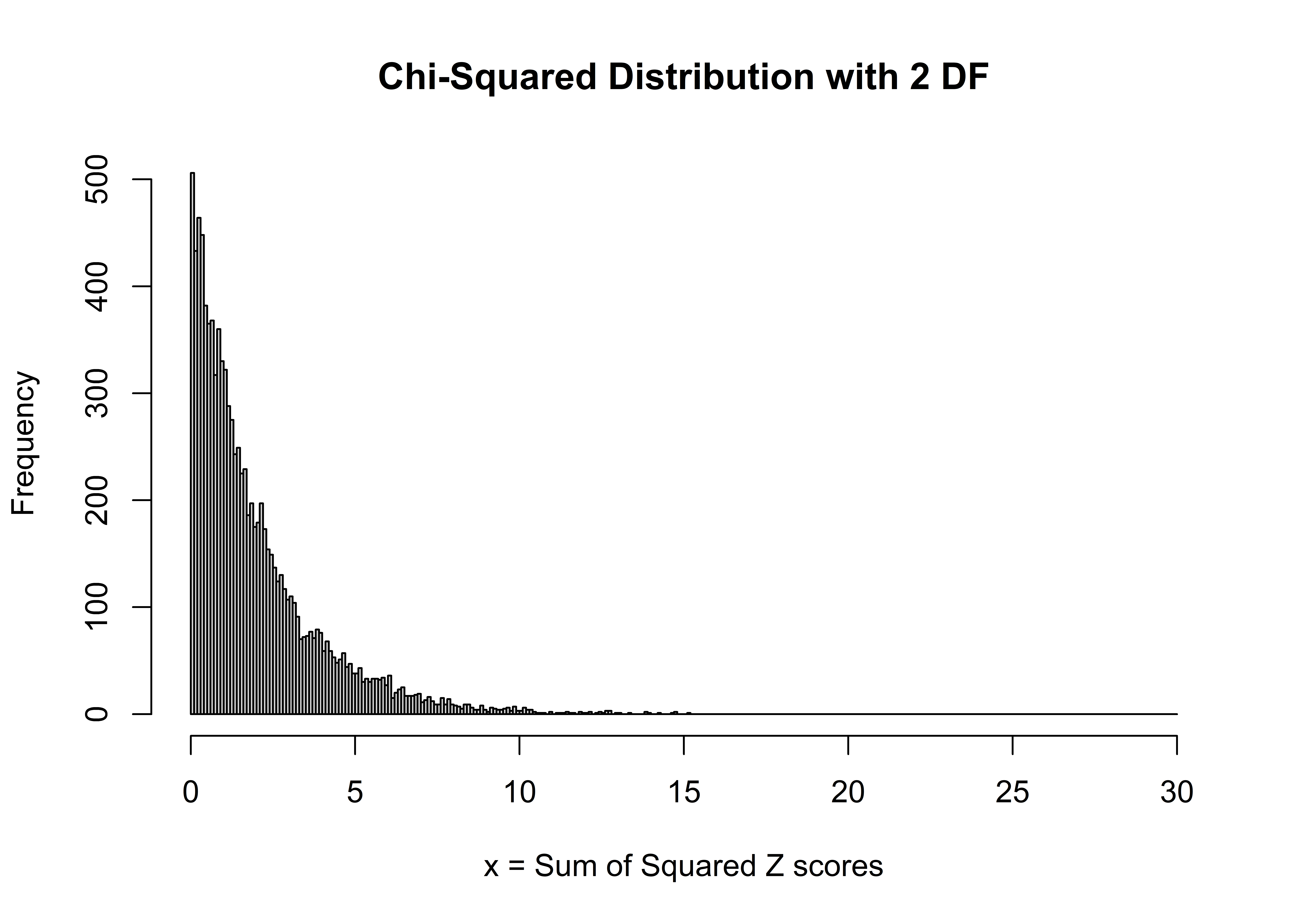
R’s vectorization methods make these easy to create, and you can continue to make “home-made” chi-squared distributions with various degrees of freedom at will.
9.2.1 dchisq
You certainly don’t need to make “home-made” distributions, but this process does drive home the message of randomness (drawing random z scores and squaring them). Nobody really makes home-made distributions. Instead, the dchisq function will provide it for you. Let’s look at the helpfile:
The arguments here are x, a vector of values to evaluate, and df, the degrees of freedom - you must indicate which chi-square distribution you’d like. For example, do you want the chi-square distribution with 1 df, or 2? Let’s use the dchisq function to plot the theoretical chi-square distribution with 2 degrees of freedom. We’ll first re-create our home-made histogram by setting the freq argument to FALSE. This “normalizes” the histogram so that the sum of the bars is equal to 1 (and the y-axis is then labeled “Density”). Then, we’ll use the lines function to overlay the theoretical chi-square distribution, colored in blue:
x <- seq(from = 0, to = 30, by = 0.1)

# generate a chi-squared distribution with 2 df as the frequency of the squared z scores
hist <- hist(sum.sq.z.scores,
     breaks = 0:30,
     xlab = "x = Sum of the Squared Z scores",
     main = "Chi-Squared Distribution with 2 DF",
     freq = FALSE)


# add a line to the histogram to show the theoretic chi square, df = 2
lines(x = 0:30, y = dchisq(0:30, df = 2),
      col = 'blue',
      lwd = 3)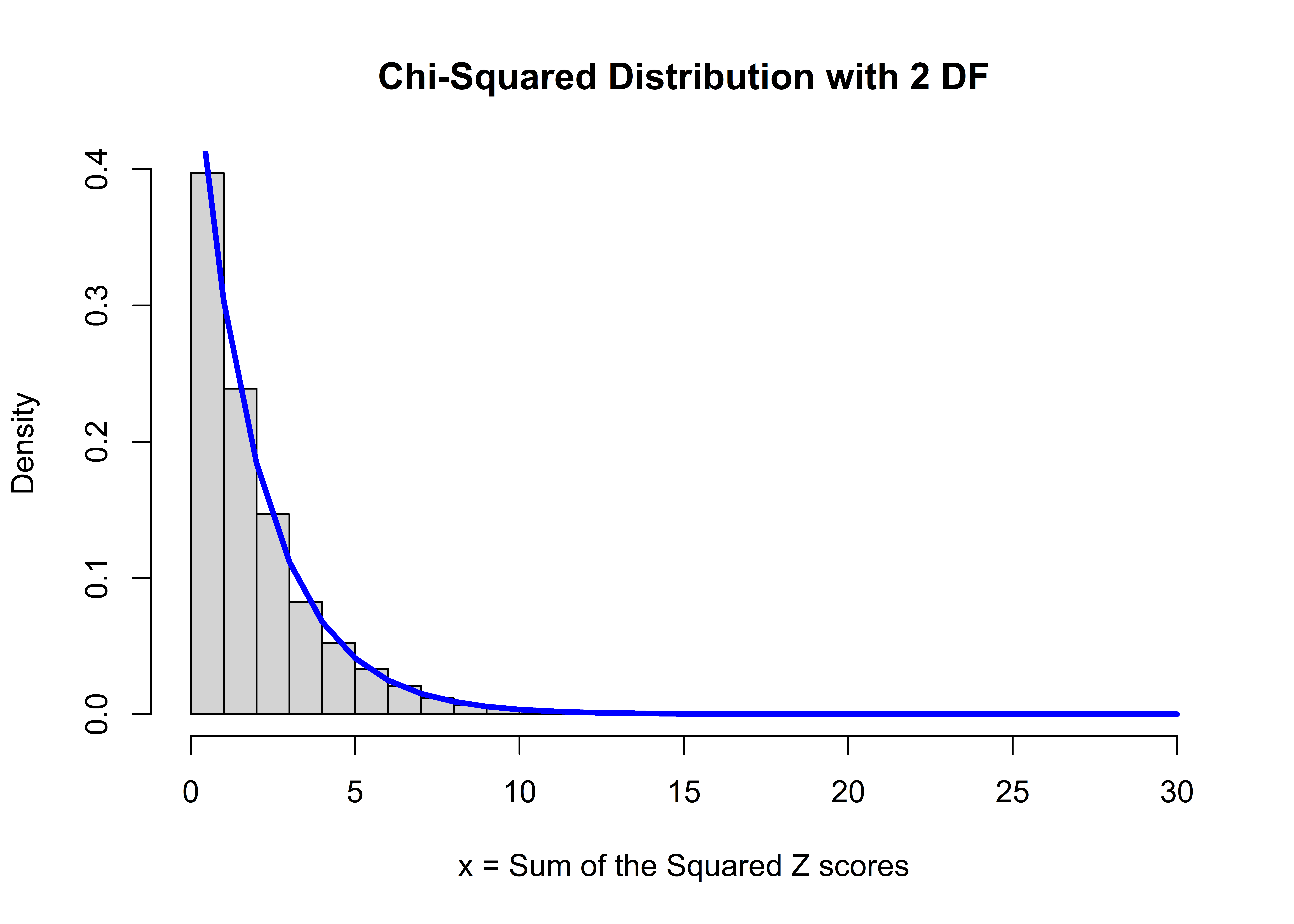
Not bad! The theoretical chi-squared distribution is a distribution whose x-axis ranges from 0 to infinity, and the shape of the distribution is controlled by one parameter called the degrees of freedom. There’s nothing magical about this distribution . . . it’s formed by adding two randomly drawn squared z scores. (The formal, theoretical chi-square distribution is a mathematical representation of this process. You can read about it here). You can see that most of the x values (sum of the squared z scores) are between 0 and 8ish, and very few values are greater than 9 or 10. Notice that all chi-square distributions start at 0 . . . you can’t have a negative result due to the squaring.
Let’s look at how the distribution changes shape as we change the degrees of freedom. First, we’ll use the plot function to plot our first distribution (df = 1). Then, once again, we’ll use the lines function to add lines to our plot.
# df = 1
plot(x = 0:30, y = dchisq(0:30, df = 1),
      lwd = 3, type = 'l', col = 'red',
      ylab = "density",
      main = "Chi-Square Distributions with Varying Degrees of Freedom")

# df = 2
lines(x = 0:30, y = dchisq(0:30, df = 2), lwd = 3, col = 'blue')

# df = 3
lines(x = 0:30, y = dchisq(0:30, df = 3), lwd = 3, col = 'green')

# df = 4
lines(x = 0:30, y = dchisq(0:30, df = 4), lwd = 3, col = 'yellow')

#df = 5
lines(x = 0:30, y = dchisq(0:30, df = 5), lwd = 3, col = 'orange')

# add a legend
legend(legend = c(1:5),
       x = "topright",
       fill = c("red","blue", "green", "yellow", "orange"))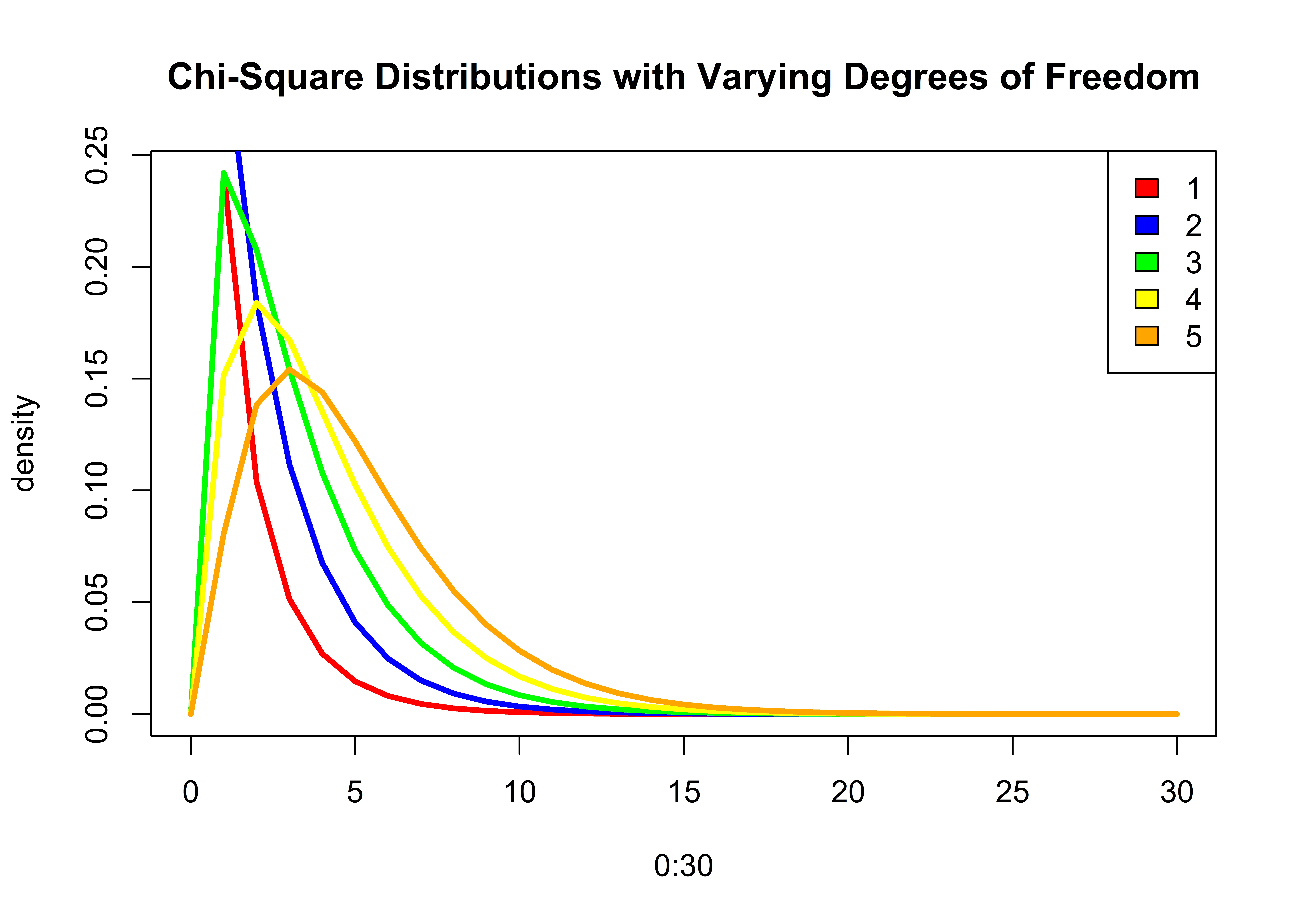
The main point here is that there isn’t just one chi-squared distribution ….there are many. The shape of the distribution is controlled by a single parameter called degrees of freedom.
9.2.2 rchisq
R has many functions for working with different kinds of statistical distributions, and these functions generally start with the letter d, p, q, or r, followed by the distribution name.
For example, if we want to draw 10 random values from a chi-squared distribution with 2 degrees of freedom, use the rchisq function. The first argument, n, provides the number of random values you’d like. The second argument, df specifies which chi-square distribution we are talking about:
## [1] 0.16794262 0.46390459 1.32733531 0.03568094 3.87815733 1.82423739 0.65297465 1.96739464 1.26679396 0.64593180Run this same bit of code again, and you’ll get a new set of random values:
## [1] 2.24911993 3.73190235 1.38927789 0.36563679 1.56116124 0.27083566 0.02683779 0.19530028 0.13288040 2.287312199.2.3 qchisq
If we want to find what x value is in the 5th percentile (quantile) for a chi-squared distribution with 2 degrees of freedom, use the qchisq function:
## [1] 5.991465The answer tells us that 95% of the ordered x values from this distribution are to the left of 5.9914645, and 5% of the X values are to the right of 5.9914645. Let’s confirm this with a plot. Here, we plot the chi-square distribution with 2 df, and use the abline function to add a vertical bar at the upper (right) tail:
plot(x = 0:20, y = dchisq(0:20, df = 2),  type = "l", lwd = 3, col = 'blue',
     ylab = "density", xlab = "x",
     main = "Chi-Square Distribution 2 Degrees of Freedom")

# add a vertical line at the 0.05 upper (right) tail
abline(v = qchisq(0.05, df = 2, lower.tail = FALSE), lty = "dashed")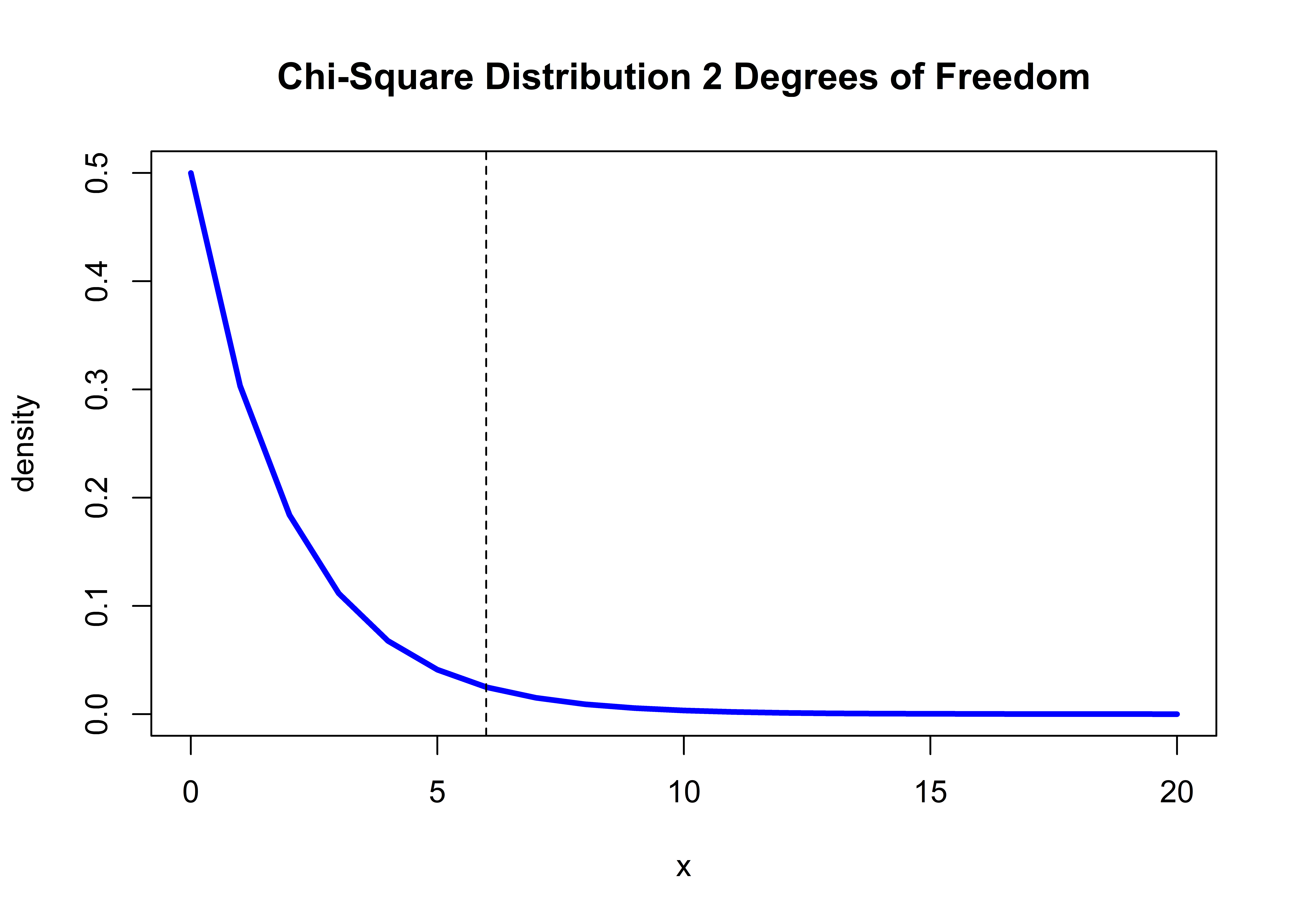
The bulk of the distribution (95%) is to the left of the dashed line. Watch that lower.tail argument! If we want to find the value of x at the lower 5th percentile, we would set the lower.tail argument to TRUE:
## [1] 0.1025866The answer tells us that 95% of the ordered x values from this distribution are to the right of 0.1025866, and 5% of the X values are to the left of 0.1025866. Let’s confirm this with a plot once more, adding a vertical bar at the lower (left) tail:
plot(x = 0:20, y = dchisq(0:20, df = 2), lwd = 3, type = "l", col = 'blue',
     ylab = "density", xlab = "x", main = "Chi-Square Distributions with df = 2")

# add a vertical line at the 0.05 lower (left) tail
abline(v = qchisq(0.05, df = 2, lower.tail = TRUE), lty = "dashed")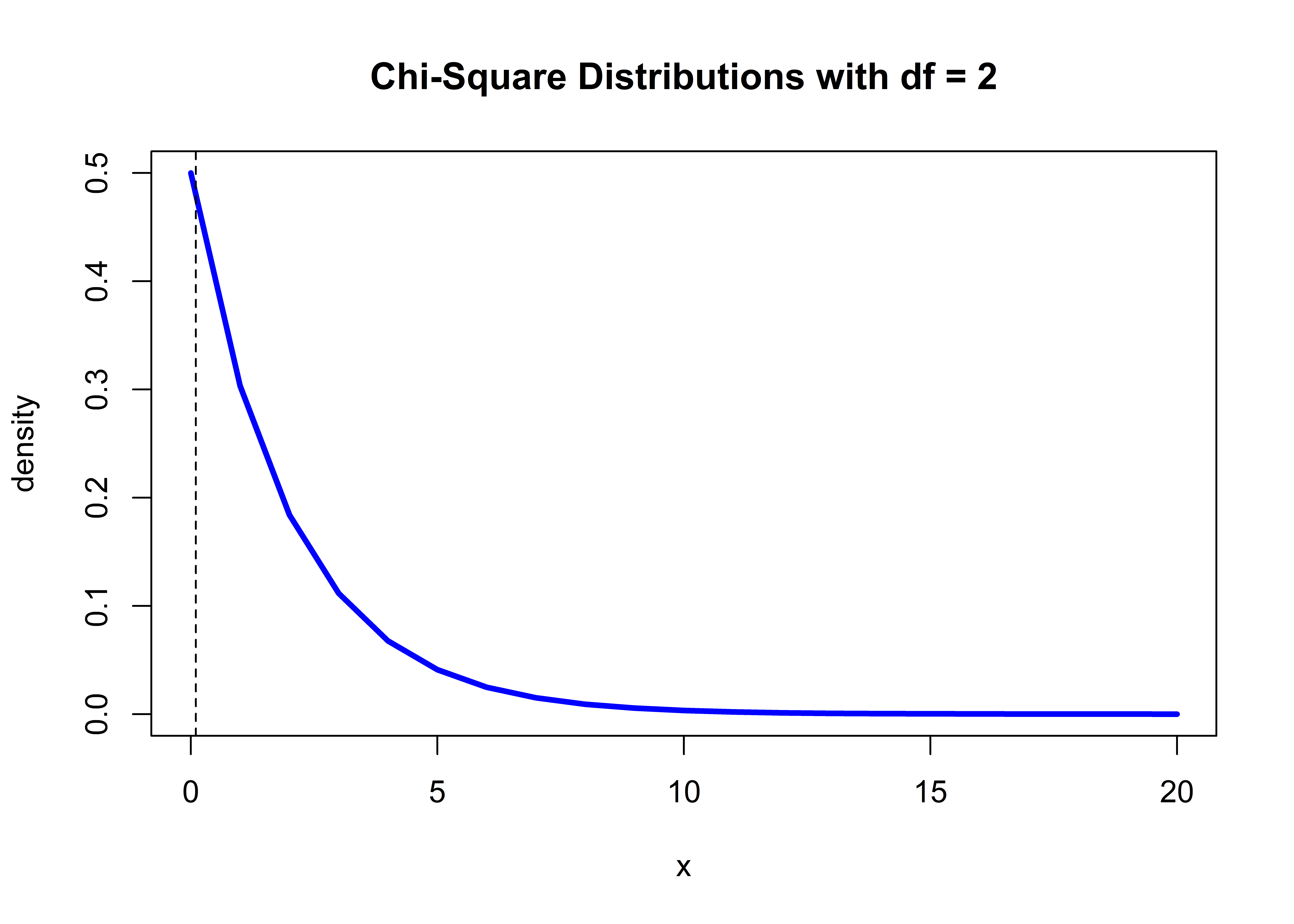
Fledglings, watch your tail! A lower tail is the left side of the distribution, while an upper tail is the right side of the distribution. Many statistical functions in R have a default value for a tail argument, and you must be aware of these settings!
9.2.4 pchisq
Returning to our voter problem, we obtained a chi-squared test statistic of 30.07, and are told now to find where this test statistic falls (percentile) on a theoretical chi-squared distribution with 2 degrees of freedom. We have the reverse information as we did before: Now we have a value of x, and we wish to know what percentage of the distribution falls above or below this value. Here, use the pchisq function, and again be mindful of the lower.tail argument:
# turn off scientific notation in R options
options(scipen = 999)

# use pchisq to find the percentile associated with 30.07
pchisq(30.07, df = 2, lower.tail = FALSE)
## [1] 0.0000002953809The answer tells us that 0.0000003 of the ordered X values from this distribution are to the right of 30.1.
What happens when we set the lower.tail argument to TRUE?
## [1] 0.9999997The answer here tells us that 0.9999997, or ~ 100% of the ordered X values from this distribution are to the left of 30.07. So our observed value is way, way out there in the right hand tail of the chi-square distribution with 2 degrees of freedom.
Let’s plot this. Our observed chi-square value is so large that we’ll need to expand the x-axis to show it!
plot(x = 0:40, y = dchisq(0:40, df = 2), lwd = 3, type = "l", col = 'blue',
ylab = "density", xlab = "x", main = "Chi-Square Distribution with df = 2")
# add a vertical line at the observed chi-square value
abline(v = 30.07, lty = "dashed")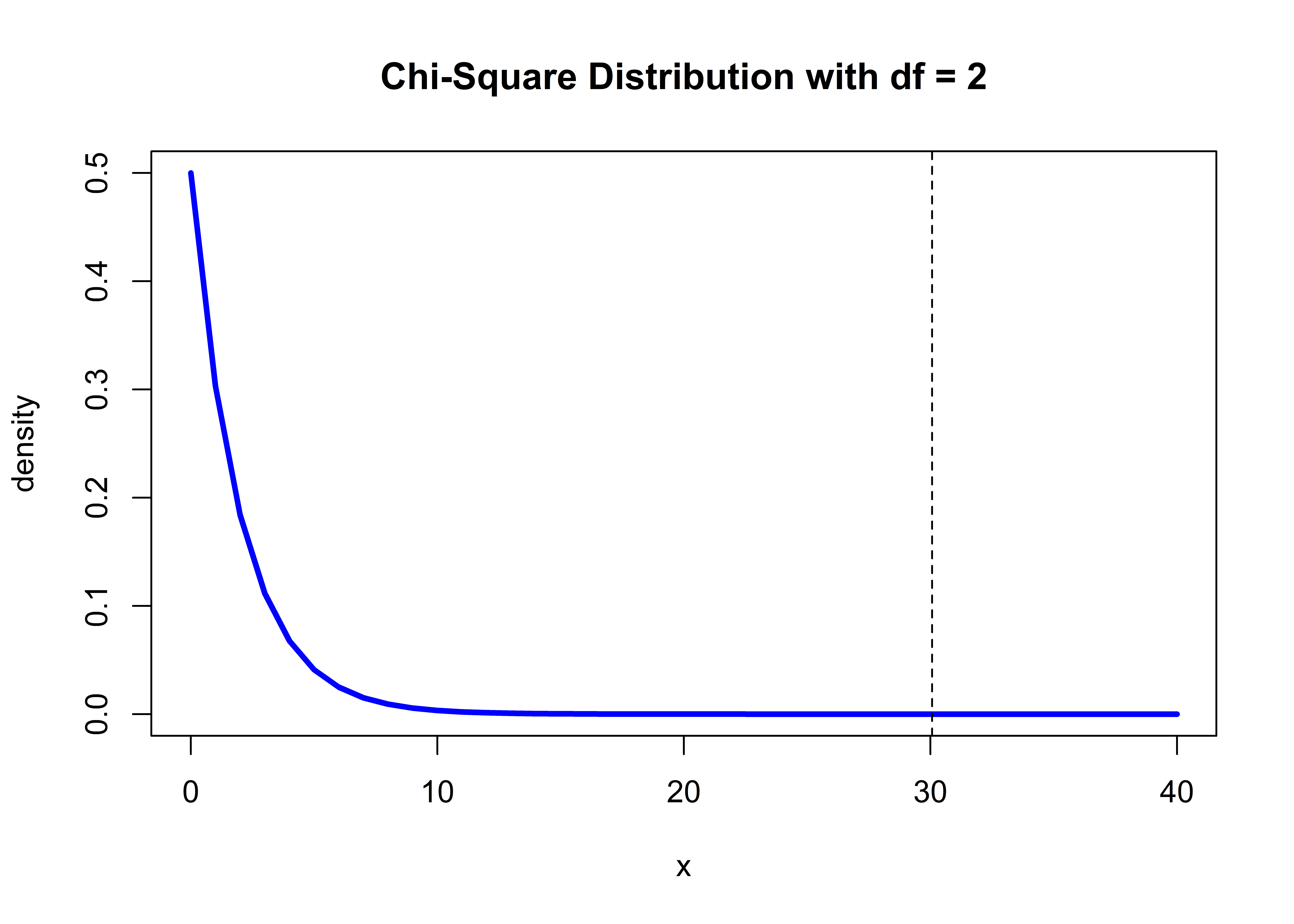 This plot shows the location of our observed value on a chi-square distribution with 2 degrees of freedom.
9.2.5 Frequentist Approaches
Almost all (frequentist) statistical tests work this same way:
- Conduct a statistical test, which returns a test statistic (here, our observed test statistic was 30.1).
- Find where this test statistic falls on a specific theoretical distribution (here, we are looking at the theoretical chi-square distribution with 2 degrees of freedom).
- Draw inferences (conclusions) based on this information.
This scientific process is known as the “frequentist method of hypothesis testing”, and has been the predominant method of statistical testing in the 20th century. See wikipedia for a general discussion. An alternative approach involves Bayesian inference, which we won’t cover here . . . check out our primer on Bayesian approaches here if you are interested.
Generally speaking, if an observed test statistic (like 30.1) is located at an extreme end of a theoretical distribution, we deem that value “unlikely” to have occurred by chance alone, and we say that our result is statistically significant. After all, we’ve shown that the chi-square distribution itself is made summed, squared random z scores. For a chi-squared test, we are only interested in values in the right tail, and our result of 30.1 is very unlikely to have arisen by chance alone. Our conclusion, therefore, is that the voter party and voter sex are NOT independent . . . the chance of observing a test statistic of 30.1 is very unlikely to have arisen by chance alone.
9.2.6 chisq.test
With that overview, at long last we are ready for the R help file example. We will simply copy and paste the first example from the chi-squared help file below (with added a few comments along the way).
We’ll first create a table called M that contains gender and political data. Many statistical functions can accept tables (a bonefide R class), as well as other formats like vectors and matrices, as arguments. We like tables in this case because the data being evaluated are very clearly identified.
# Copy chi-squared test example from help files
M <- as.table(rbind(c(762, 327, 468), c(484, 239, 477)))
dimnames(M) <- list(gender = c("M","F"),
                    party = c("Democrat","Independent", "Republican"))

# look at the table M
M
## party
## gender Democrat Independent Republican
## M 762 327 468
## F 484 239 477M is an R object of class “table”. These are the same values we showed at the beginning of the chapter. Now, let’s run the chi-square test with the chisq.test function. We just need to pass in M, and R will do the rest.
##
## 	Pearson's Chi-squared test
##
## data:  M
## X-squared = 30.07, df = 2, p-value = 0.0000002954
You should see that these results match our boxes a-e above (except for the number of decimal places displayed). The section data: M specified that our data is called M. The value X-squared = 30.07 gives our test statistic. The p value returned is the same as what was returned by the pchisq function, and we take this to indicate what percentage of the distribution falls to right of our our observed value
## [1] 0.0000002953809Keep in mind you can run an analysis and not store the result as an object, as we’ve just seen. However, there is no way to easily retrieve all of the results! For that reason, most of the example R helpfiles have you store the results as an object, and this object usually is a list. We’ll explore this more next.
Let’s get back to our Tantaun research question and create an object using the table function to summarize fur length and fur color.
table.lengthcolor <- table(TauntaunData$color, TauntaunData$fur)

# show the new object
table.lengthcolor
##
## Short Medium Long
## White 1293 1263 1296
## Gray 3121 3071 3308Now, we can use this table as an input to the chisq.test function to test whether Tauntaun fur length and fur color are related, using the chisq.test function. This time, we’ll store the results of this analysis as a new object called “chisq.result”.
# run the analysis and store the result as chisq.result
chisq.result <- chisq.test(table.lengthcolor)

# show the result
chisq.result
##
## Pearson's Chi-squared test
##
## data: table.lengthcolor
## X-squared = 1.7027, df = 2, p-value = 0.4268Can you find this value on the Chi-Square Distribution? Remember to use the distribution with 2 degrees of freedom.
plot(x = 0:40, y = dchisq(0:40, df = 2), lwd = 3, type = "l", col = 'blue',
ylab = "density", xlab = "x", main = "Chi-Square Distribution with df = 2")
# add a vertical line at the observed chi-square value
abline(v = 1.7027, lty = "dashed", col = "red")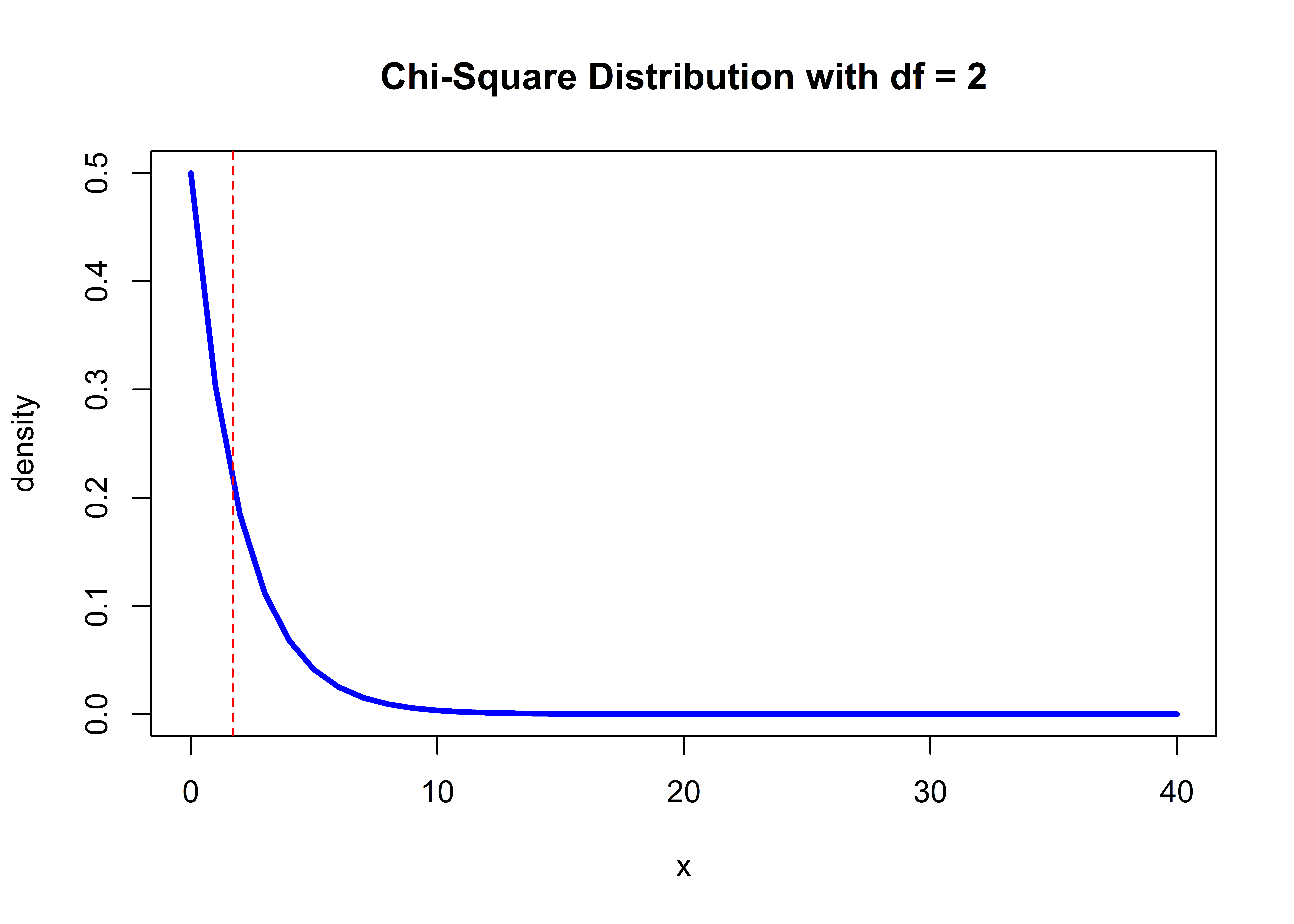
What’s conclusions (inferences) can you draw? Here, our observed chi-square value for Tauntauns falls squarely in the thick part of the theoretical chi-square distribution with 2 degrees of freedom. We’re pretty likely to observe that value even by chance (remember our squared random z values?). In this case, we would conclude there is not sufficient evidence that Tauntaun fur length and fur color are associated in any way.
Let’s take a few minutes to examine the output of the chi-squared test. The first thing to notice is that only portions of the result are returned to the console. To find what’s under the hood, look for chisq.result in your global environment. You’ll see that it is an htest object type (which we assume stands for a hypothesis test), with a value of “list of 9” (check the RStudio global environment). Several statistical tests in R result in htest object types. This object type is a list that records all of the information about the test that you performed. In the case of the chi-squared test, there are 9 pieces of information that result from the test. Use the str function to see the details.
## List of 9
## $ statistic: Named num 1.7
## ..- attr(*, "names")= chr "X-squared"
## $ parameter: Named int 2
## ..- attr(*, "names")= chr "df"
## $ p.value : num 0.427
## $ method : chr "Pearson's Chi-squared test"
## $ data.name: chr "table.lengthcolor"
## $ observed : 'table' int [1:2, 1:3] 1293 3121 1263 3071 1296 3308
## ..- attr(*, "dimnames")=List of 2
## .. ..$ : chr [1:2] "White" "Gray"
## .. ..$ : chr [1:3] "Short" "Medium" "Long"
## $ expected : num [1:2, 1:3] 1273 3141 1250 3084 1328 ...
## ..- attr(*, "dimnames")=List of 2
## .. ..$ : chr [1:2] "White" "Gray"
## .. ..$ : chr [1:3] "Short" "Medium" "Long"
## $ residuals: 'table' num [1:2, 1:3] 0.549 -0.349 0.358 -0.228 -0.885 ...
## ..- attr(*, "dimnames")=List of 2
## .. ..$ : chr [1:2] "White" "Gray"
## .. ..$ : chr [1:3] "Short" "Medium" "Long"
## $ stdres : 'table' num [1:2, 1:3] 0.795 -0.795 0.516 -0.516 -1.295 ...
## ..- attr(*, "dimnames")=List of 2
## .. ..$ : chr [1:2] "White" "Gray"
## .. ..$ : chr [1:3] "Short" "Medium" "Long"
## - attr(*, "class")= chr "htest"All htest objects contain at least one element called statistic (value of the test statistic) and one element called p.value (value of the p-value, or the percentile of the test statistic on the theoretical distribution). To extract those values, you can use any of the list subsetting methods we learned in previous chapters (because the htest object type is a list) and as illustrated in the helpfile example. For instance, as the Tauntaun biologist, if you want to report that there is no association between fur length and fur color and report the p-value, you can pull out the p-value like this:
## [1] 0.4268283Take time now to poke into each element of this list!
9.2.7 Methods
In R, a function that works on a particular class of R objects is called a “method”. The methods function will return a list of methods for an object of a given class. This is a handy function to know and is worth trying on the statistical outputs you generate. For example, the following code will ask R to return a list of methods that can be used on objects of class “htest”.
## [1] print
## see '?methods' for accessing help and source codeYou can see that only one method is displayed here (we’ll see a better example of this soon). Let’s see what the print method does if we pass in our chisq.result object:
##
## 	Pearson's Chi-squared test
##
## data:  table.lengthcolor
## X-squared = 1.7027, df = 2, p-value = 0.4268Hopefully you are getting the gist of running of statistical analyses in R. Next, we’ll run through three more commonly used statistical analyses, the t-test, correlation, and regression. Though the analytical framework will differ, the basic steps will be the same.
- Data are fed into the statistical function.
- An observed test statistic is generated.
- We find where that test statistic falls on a theoretical statistical distribution.
- We draw conclusions based on that result.
In running any statistical function in R, the steps you should remember are:
- Identify the function needed.
- Read the help page.
- Execute the examples in the help page with the
examplefunction. - Use the
strfunction on the sample output so that you can determine what sort of object the analysis returns. This is crucial for prying information out of the object (pulling the result out of the shoebox).
We will follow these steps for our next analyses. However, we promise not to drag you through the theoretical statistical distributions, so the rest of the chapter should go quickly! First, let’s have a quick break.
Figure 9.2: Ahhh! That’s better!
9.3 T-test
As you can imagine, comparing two groups is one of the most basic problems in statistics. One of the easiest ways to compare the means of two groups is by using a t-test. According to Wikipedia, the t-test was introduced in 1908 by William Gosset,a chemist working for the Guinness brewery in Dublin, Ireland.
Let’s use a t-test to ask whether mean length of male Tauntauns differs from the mean length of female Tauntauns. But before we do that, let’s first look at the help files and arguments for the function t.test:
## function (x, ...)
## NULL
The args function isn’t too helpful here, but the help files cover arguments, additional details about the function, output values, and examples, as usual. Here, we notice a very important similarity with the chi-squared output - they are both htest objects with several elements in a list.
What should we do first to examine this function in detail? Great idea - let’s run an example from the help file. The example we’ll focus on here is a t-test of Student’s Sleep Data. This is a built-in dataset from R (included in the package, datasets), and it has just a few columns. Let’s take a look:
##   extra group ID
## 1   0.7     1  1
## 2  -1.6     1  2
## 3  -0.2     1  3
## 4  -1.2     1  4
## 5  -0.1     1  5
## 6   3.4     1  6
In case you are curious about the built-in ‘sleep’ dataset, use the
helpfunction, and type help(package = datasets), and then search for the dataset of interest in the help file (in this case the dataset is called sleep). The datasets package comes with the base program and are already loaded when you open R, so you do not need to load them with thelibraryfunction.
Ok, now back to the t-test example. We were just about to look at the columns in the example dataset. You should see three columns: ‘extra’, ‘group’, and ‘ID’. Extra is the change in hours of sleep (a numeric datatype); group is the drug given (a factor datatype); ID is the individual patient ID (a factor datatype). Here, we want to know whether a change in hours of sleep is a function of group. Specifically, we want to know if the mean hours of sleep for group 1 is different than the mean sleep hours of group 2. We can use the aggregate function to see what the means are of the two groups:
##   group extra
## 1     1  0.75
## 2     2  2.33
Well, of course these values are different! Why run a statistical analysis? Because the sleep dataset consists of samples, and the values shown above may be very different if we had evaluated a different set of patients. We need to account for this sample-to-sample bias that arises when we can’t measure all sleep patients. That’s what statistics is all about – drawing conclusions based on information stored in samples.
9.3.1 The Classical Interface
There are two ways to run a t-test in R: the classical interface and the formula interface. Here, we’ll follow the code in the Student’s Sleep Data under the classical interface example. First, let’s simply plot the data by group:
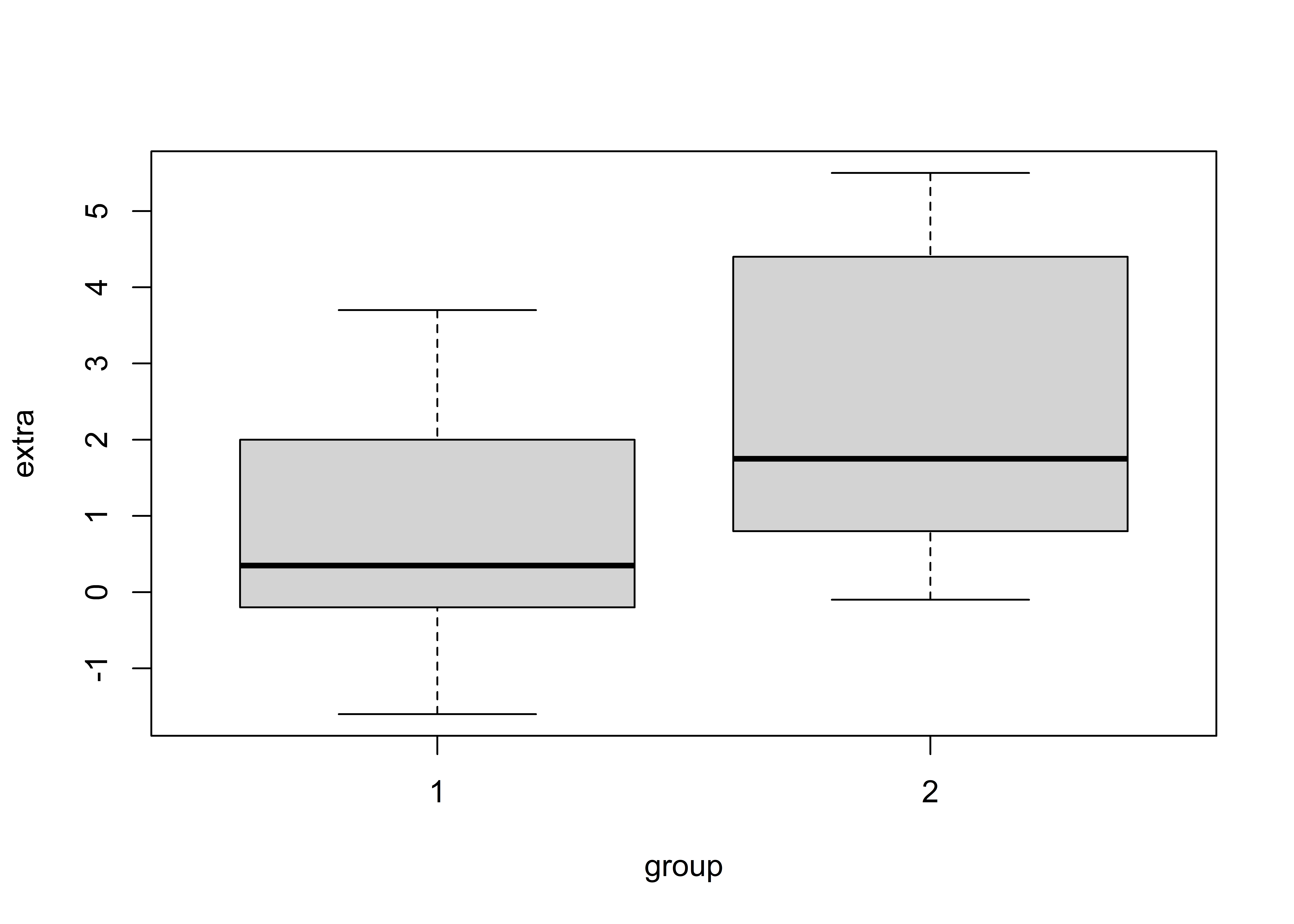
Figure 9.3: Boxplot of the two sleep groups.
This plot is showing the change in sleep hours for each of the two groups that were administered different drugs. This is a nice boxplot visual that gives us information about the range of the raw data in each group and the median values (identified by the thick horizontal lines). But we don’t care about the raw data - our goal is to compare the two group means statistically, and to do that we need to run a t-test.
Copy and paste the second example from the t.test help file, called the traditional interface example.
##
## 	Welch Two Sample t-test
##
## data:  extra[group == 1] and extra[group == 2]
## t = -1.8608, df = 17.776, p-value = 0.07939
## alternative hypothesis: true difference in means is not equal to 0
## 95 percent confidence interval:
##  -3.3654832  0.2054832
## sample estimates:
## mean of x mean of y
##      0.75      2.33
Did you notice the code notation using the with function? This function provides a little bit of shorthand to make the subsetting process easier. It first tells R that we are working with the sleep dataset, so that any following notation is assumed to refer to that same dataset. (This is handy if you don’t like using $ signs to reference columns . . . some people think this results in cleaner code.)
The t.test function in this example has two arguments, extra[group == 1] and extra[group == 2]. These represent the two vectors of data that we are interesting in comparing.
In the output of this t.test example (above), we see references to the two numeric vectors representing arguments x and y - the two groups being analyzed. The test statistic is called t, and it has a value of t = -1.8608. To understand how to interpret the test statistic, we need to find where this value falls on a t-distribution that has 17.776 degrees of freedom. Thus, the t-distribution is defined by a single parameter called degrees of freedom (as in the chi-square distribution).
The sleep dataset has 10 observations in group 1, and 10 observations in group 2. Typically, the degrees of freedom is calculated based on the number of samples in each group (minus 1), added together. In this case, would be (10-1) + (10-1) = 18. What’s with the 17.766?
Fledglings, always check the default arguments!
The t.test argument called var.equal has a default of FALSE, so the Welch (or Satterthwaite) approximation to the degrees of freedom is used (which is why you see the name Welch in the output). This default value is hard to find . . . it’s in the Details section of the helpfile). If we were to run this again and set the var.equal argument to TRUE, we would get a result that you may have been expecting (a t-distribution with 18 degrees of freedom).
## Traditional interface
with(sleep, t.test(extra[group == 1], extra[group == 2], var.equal = TRUE))
##
## Two Sample t-test
##
## data: extra[group == 1] and extra[group == 2]
## t = -1.8608, df = 18, p-value = 0.07919
## alternative hypothesis: true difference in means is not equal to 0
## 95 percent confidence interval:
## -3.363874 0.203874
## sample estimates:
## mean of x mean of y
## 0.75 2.33Like the chi-square distribution, the shape of the t distribution is controlled by one parameter called the degrees of freedom; but it is not generated with z scores! You can learn more about this distribution on Wikipedia at http://en.wikipedia.org/wiki/Student's_t-distribution, but for now, here’s a quick look at a few t-distributions that vary in their degrees of freedom:
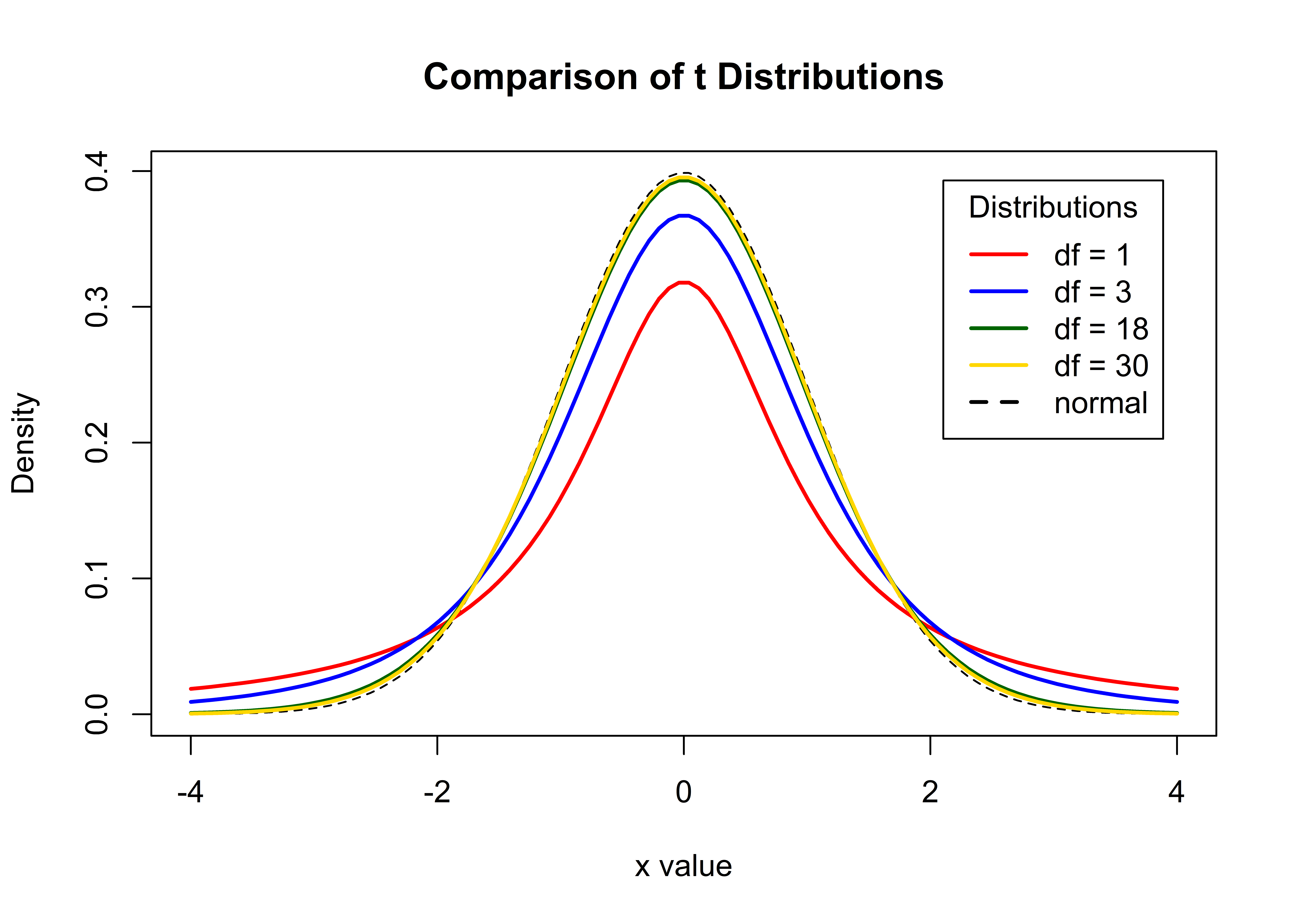
Notice that as the degrees of freedom increases (as sample size increases), the t-distribution becomes more and more like the standard normal distribution. With smaller sample size, the tails of the distribution are fatter.
For the sleep data, we need to determine where our observed test statistic value falls on a t-distribution that has 17.776 degrees of freedom . . . which is close to the green-shaded distribution in the figure above.
Now, here’s the kicker . . . are you interested in test statistic results that fall in the right tail only? Are you interested in test results that fall in the left tail only? Or are you interested in results that fall in either tail? The example we ran assumes a two-tailed test, meaning that we are interested in finding out if our observed test statistic falls in either tail. If you want to run a one-tailed t test, you can set the argument alternative to “less” or “greater”, depending on which tail you are interested in.
Just like the chi-square distribution, R has several functions for exploring a given t distribution. Remember that these begin with the letters d, p, q, or r, followed by the letter t (for t distribution). Let’s try a few.
9.3.2 qt
If we want to find what x value is in the 2.5 and 97.5 percentile (quantile) for a t-distribution with 18 degrees of freedom, use the qt function:
## [1] -2.100922 2.100922By passing in a vector c(.025, .975) for the argument called p, R returns the values associated with both the 0.25 and 0.975 percentiles. With the lower.tail argument set to TRUE, the answer tells us that 2.5% of the ordered X values from this distribution are to the left of -2.100922, and 97.5% of the X values are to the left of 2.100922.
9.3.3 pt
If we have an observed t-test statistic of -1.8608, and want to find where this statistic falls (percentile) on a t-distribution with 18 degrees of freedom, we use the pt function.
# return proportion of the t distribution that fall to the right of x = -1.861
pt(-1.8608, df = 18, lower.tail = FALSE)## [1] 0.9604056# return proportion of the t distribution that fall to the left of x = -1.861
pt(-1.8608, df = 18, lower.tail = TRUE)## [1] 0.03959435The R stats functions that begin with the letter p are the ones you’d likely use to find your p value (which percentile is associated with your observed test statistic.)
9.3.4 rt
To generate random values from a t-distribution with a specified degrees of freedom, us the rt function. The argument n specifies how many values to draw, and the argument df specifies which t-distribution you are talking about:
## [1] 0.4660087 0.3090475 -0.4621386 1.7425706 -1.0783635 0.5263814 1.1313095 -0.7037305 -0.3554921 2.2300169Now let’s look back to what the t.test function actually returned for the sleep data, and see if we can find these same results.
##
## 	Two Sample t-test
##
## data:  extra[group == 1] and extra[group == 2]
## t = -1.8608, df = 18, p-value = 0.07919
## alternative hypothesis: true difference in means is not equal to 0
## 95 percent confidence interval:
##  -3.363874  0.203874
## sample estimates:
## mean of x mean of y
## 0.75 2.33The p-value returned is 0.07919. This result is intended to help you draw conclusions on whether the sleep drug worked or not. Researchers often use the magical value of 0.05 (sometimes referred to as ‘alpha’) as a “cutoff” for concluding whether the test was “statistically significant”. If we used this cutoff, our observed test statistic of t = -1.8608 does not fall far enough into the tails of a t-distribution with df = 17.776, so we would claim that there is not sufficient evidence to conclude the sleep drug worked.
But . . . where does 0.07919 come from? It has to do with the fact that we are running a two-tailed t-test. Here, we are looking for results in the far left hand tail or the far right hand tail, and specifically are interested in values in the 2.5 percentile on either tail. Since the distribution is symmetrical, we can find our result as:
lower.tail  <- pt(-1.8608, df = 18, lower.tail = TRUE)
upper.tail  <- pt(-1.8608, df = 18, lower.tail = TRUE)
p.value  <- lower.tail + upper.tail
p.value
## [1] 0.07918871As mentioned above, the results of all htest objects contain at least one element called statistic (value of the statistic) and one element called p.value (value of the p-value). We see those values output several times corresponding to different inputs.
9.3.5 The formula interface
Now, we’ll copy and paste the third Student’s Sleep Data example (formula interface) from the t.test help file into our R script (with argument names added). This example shows you how to use the t.test function using the formula notation instead of the classical notation. We used the formula interface in previous chapters, but let’s remind ourselves of its notation, which sets a dependent variable as a function of independent variables. Here, the dependent variable extra is a function of (~) the independent variable, group.
##
## 	Two Sample t-test
##
## data:  extra by group
## t = -1.8608, df = 18, p-value = 0.07919
## alternative hypothesis: true difference in means is not equal to 0
## 95 percent confidence interval:
##  -3.363874  0.203874
## sample estimates:
## mean in group 1 mean in group 2
##            0.75            2.33
You can see that the results are the same as the classic notation, but the output looks a bit different. The formula notation’s output identifies the group name (in this case ‘group 1’ or ‘group 2’), while the classical notation retains the x and y generic arguments. Remember, formula notation is very common for many different statistical tests.
Finally, a quick note about saving the results of your statistical tests as objects: in the t.test examples, we are not saving the results. Therefore, you are unable to extract the pieces of the results. To pull out the results, simply assign them to an object like we did with the chi-squared test. We will practice this more below.
Let’s get back to the Tauntaun research question: is there a difference in the mean weight of male and female Tauntauns? Here, we’ll analyze just one year’s worth of data, say 1901. Choose a t.test notation technique based on the examples we just went through and create an object for your results, then look at the structure of the new object:
# subset TauntaunData data for a given year
annual.harvest  <- subset(x = TauntaunData, year == 1901)

# run a t test to determine if weight varies by sex
ttest.results  <- with(annual.harvest, t.test(weight[sex == 'm'], weight[sex == 'f']))

# show the t-test results
ttest.results
##
## Welch Two Sample t-test
##
## data: weight[sex == "m"] and weight[sex == "f"]
## t = 29.131, df = 865.22, p-value < 0.00000000000000022
## alternative hypothesis: true difference in means is not equal to 0
## 95 percent confidence interval:
## 219.5347 251.2544
## sample estimates:
## mean of x mean of y
## 992.1662 756.7716## [1] "statistic" "parameter" "p.value" "conf.int" "estimate" "null.value" "stderr" "alternative" "method" "data.name"Notice again that the returned object is an htest object with a list of 10 elements including statistic and p.value. Here, you can also see the argument alternative is set to two.sided. Use your list extraction techniques to pull out any elements from ttest.results.
The final step of this analysis is interpreting the results. Our t-statistic = 29.131 with 865.22 degrees of freedom has a p-value of nearly 0. What can you conclude about differences in weight between male and female Tauntauns from this result? There is almost no chance that the differences between the sampled weights could have arisen by chance.
For maximum clarity, it is always useful to plot your results. In other words, don’t focus so much on the p-values as much as the effect size – the actual difference in the mean weight between males and females. That’s the real result.
If we wanted to look at the raw data, we could use the boxplot function. But here, with our t-test result, we want to focus only on the means of the two groups, and show their differences. However, we should also display the confidence intervals around our estimates of the mean. Again, although our raw data clearly shows the two means are different, we need to acknowledge that we have uncertainty in these estimates because we have used a sample (a different sample would produce different means).
The standard error of the means can be computed by hand as the standard deviation of each group divided by the sample size minus 1. Here, to save space, we’ll use the dplyr pipe approach to quickly summarize the Tauntaun data:
# load dplyr
library(dplyr)

# summarize the sleep data
harvest.summary <- annual.harvest %>%
  group_by(sex) %>%
  summarise(
    n = n(),
    mean = mean(weight),
    sd = sd(weight),
    se = sd(weight)/(n() - 1),
    .groups = 'drop')

# show the resulting tibble
harvest.summary
## # A tibble: 2 x 5
## sex n mean sd se
## <fct> <int> <dbl> <dbl> <dbl>
## 1 f 490 757. 112. 0.229
## 2 m 441 992. 132. 0.301Let’s now use this information to create a plot with ggplot2. Here, we want sex to be on the x-axis, and the y-axis will plot the mean. We’ll then use the geom_point function to plot the mean of each group as a point, and the geom_errorbar function to add error bars around the mean (+/- 1SE * 1.96). (Multiplying the standard error by 1.96 would gives us the upper and lower 95% confidence intervals around each mean). We’ll set the labels and axes limits as well.
# load ggplot2
library(ggplot2)

# plot the sleep means by group, including the standard errors
ggplot(harvest.summary, aes(x = sex, y = mean, group = 1)) +
    geom_point() +
    geom_errorbar(aes(ymin = mean - 1.96 * se, ymax = mean + 1.96 * se),  width = 0.1) +
    ylab("Mean Tauntaun Weight") +
    xlab("Sex")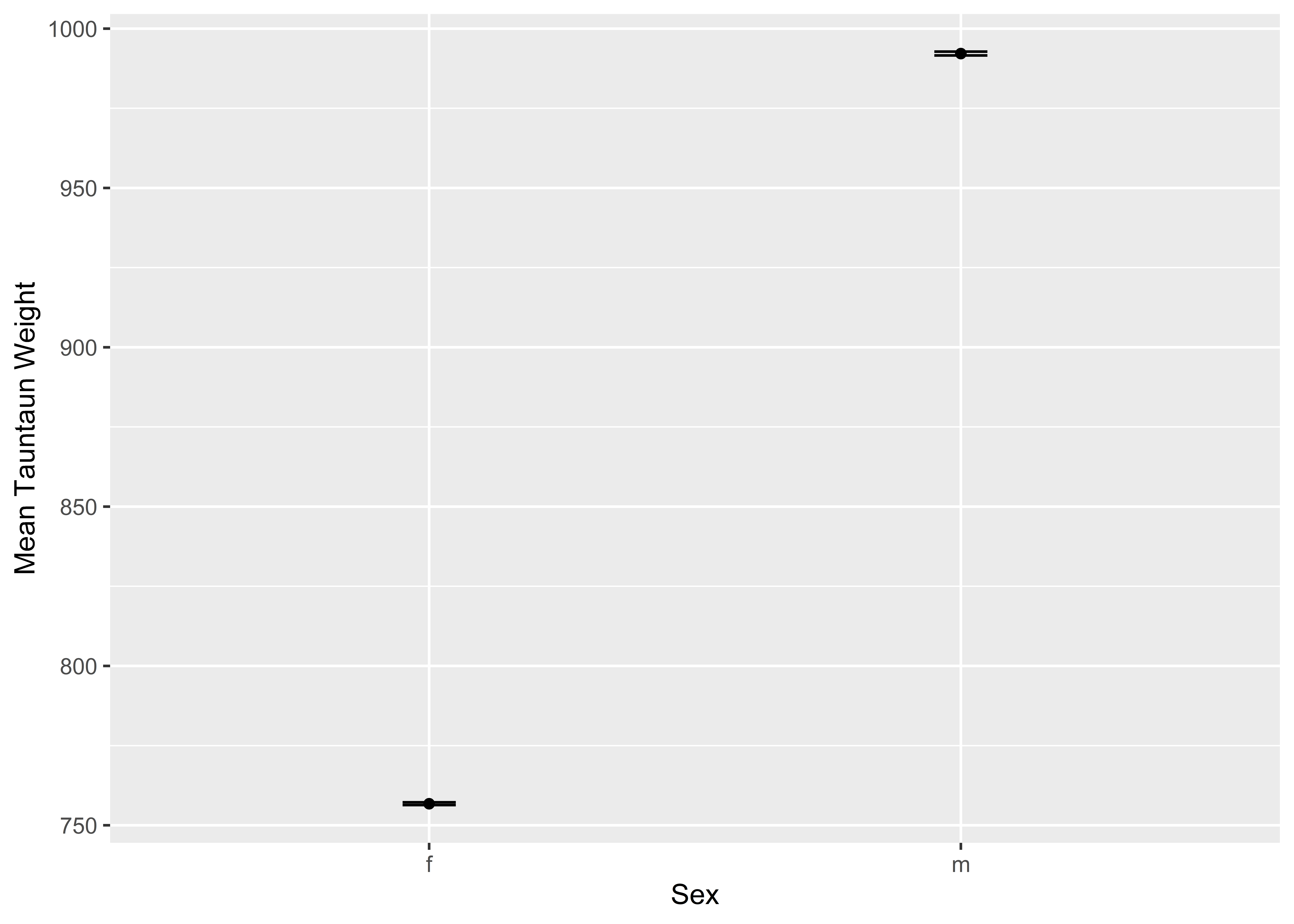
There now. This graph shows our t-test results nicely. There is no question that Tauntauns vary in weight by sex. This is not a sampling artifact. The “effect size” is the difference between the weights by group.
We’ll end our introduction to t-tests there. As with all statistical approaches, you can (and should) go deeper. We’ve blown past a few essential steps that should be taken, such as looking for outliers, testing for equal variance among groups, and other assumptions. A tutorial on t-tests using the Magritrr pipe can be found at datanovia.com.
9.4 Correlation
From here on out, we’ll be focusing on two variables that you, the Tauntaun biologist, are very interested in: length and weight.
As the Tauntaun biologist, you want to know whether there is a linear relationship between Tauntaun length and Tauntaun weight. That is, as length goes up, does weight also go up? Or maybe Tauntauns are a total anomaly, where as length goes down, weight goes up! If a relationship exists, how tight is this relationship?
The first step in the correlation process is to plot the raw data, which is easily done with the plot function. Let’s stick with our 1901 harvest data for this section.
# use the plot function to plot the weight and length data
plot(x = annual.harvest$length,
     y = annual.harvest$weight,
     main = "Tauntaun Weight as a Function of Length",
     xlab = "Tauntaun Length ", ylab = "Tauntaun Weight",
pch = 19, col = annual.harvest$sex) 
It’s pretty clear that as length increases, so does weight. So Tauntauns are not that unusual. We simulated the data so that there would be a relationship, so the authors are not surprised by this result. We’ll formally evaluate this relationship with a Pearson’s correlation analysis.
From Wikipedia, we learn that:
In statistics, the Pearson product-moment correlation coefficient (or Pearson’s r) is a measure of the linear correlation (dependence) between two variables X and Y, giving a value between +1 and -1 inclusive, where 1 is total positive correlation, 0 is no correlation, and -??1 is total negative correlation. It is widely used in the sciences as a measure of the degree of linear dependence between two variables. It was developed by Karl Pearson from a related idea introduced by Francis Galton in the 1880s.
The words “linear dependence” are crucial. If there is a strong, non-linear pattern in your data, Pearson’s r is not the correct test to use, and the cor.test function will not detect the relationship.
The cor.test function can be used to test for correlations. First, as always, look at the helpfile.
The cor.test function requires two vectors of data, which make up arguments x and y. The default method of analysis is the Pearson’s correlation. Let’s try this function now:
# run a correlation test between length and weight
cor.test(x = annual.harvest$length, y = annual.harvest$weight)
##
## Pearson's product-moment correlation
##
## data: annual.harvest$length and annual.harvest$weight
## t = 42.671, df = 929, p-value < 0.00000000000000022
## alternative hypothesis: true correlation is not equal to 0
## 95 percent confidence interval:
## 0.7908271 0.8343590
## sample estimates:
## cor
## 0.813731You can see that the data are highly correlated (by design!). Let’s run the analysis again, this time storing the result so you can extract information from it for a report (if needed).
# store the output as cor.out
cor.out  <- cor.test(x = annual.harvest$length, y = annual.harvest$weight)

# look at the list names of the output, cor.out
names(cor.out)
## [1] "statistic" "parameter" "p.value" "estimate" "null.value" "alternative" "method" "data.name" "conf.int"You can also see that males and females might be treated separately in future analyses. Remember that our data are samples only, so there will be some error associated with our estimate of the correlation coefficient. Look for the 95 percent confidence intervals to accurately report your correlation estimate. This portion of output is located in a list element called conf.int, which you can extract with [[ ]], e.g., by running the command cor.out[[‘conf.int’]].
# extract the confidence intervals for the correlation coefficient (a statistic)
cor.out[['conf.int']]
## [1] 0.7908271 0.8343590
## attr(,"conf.level")
## [1] 0.95We take this to mean: "The 95% confidence intervals for the correlation coefficient span between 0.7908271 and 0.8343590. By the way, if you have ranked data, you could specify method = ‘spearman’ to get a correlation coefficient for the ranked data.
9.5 Regression
A related statistical test is a regression analysis. You just ran the correlation test between length and weight, but now you need a tool that will let you predict a Tauntaun’s weight if you know its length Regression analysis is a statistical method that will provide this by estimating a best-fit line through the data. Here, we’ll use the lm function, which stands for ‘linear model’, to run a regression analysis. In statistics, a linear model relates a dependent variable to one or more independent variables. First, let’s look at the arguments for lm:
## function (formula, data, subset, weights, na.action, method = "qr",
##     model = TRUE, x = FALSE, y = FALSE, qr = TRUE, singular.ok = TRUE,
##     contrasts = NULL, offset, ...)
## NULL
The first argument is called formula, and here you would enter a formula similar to the t-test formula interface. For a single factor model, the formula notation is y ~ x, and can be read aloud as “y is a function of x”. This is the type of model you would use to investigate if weight is a function of length. Here, weight is the dependent variable, and length is the independent or predictor variable because it is used to predict the value of the dependent variable, weight. So to express tauntaun weight as a function of length, we write weight ~ length. (Check the help files for formula for more information on formula notation.)
The second argument is called data, where you point to the data to be analyzed. There are other arguments as well, many of which have default values that you’ll want to be familiar with before using this function.
Let’s have a look at the output:
##
## Call:
## lm(formula = weight ~ length, data = annual.harvest)
##
## Coefficients:
## (Intercept)       length
##      48.765        2.359
What do you notice about the result of this test? It is pretty short. It basically returns the function call (lm(formula = weight ~ length, data = annual.harvest)) and the coefficients. Here, we are fitting a line through our data, and a line that best “fits” the data is a line whose y-intercept is 48.765 and whose slope is 2.359. For every unit increase in length, Tauntaun weight increase by 2.359 units. These our our linear regression coefficients.
However, like other statistical outputs from R, it is crammed packed with the gory details of the analysis. Let’s look at the structure of the returned object:
## List of 12
##  $ coefficients : Named num [1:2] 48.76 2.36
##   ..- attr(*, "names")= chr [1:2] "(Intercept)" "length"
##  $ residuals    : Named num [1:931] -65.9 88.5 -15.7 -61.7 2.9 ...
##   ..- attr(*, "names")= chr [1:931] "10600" "1658" "920" "2018" ...
##  $ effects      : Named num [1:931] -26493.04 4204.24 -9.53 -63.36 10.11 ...
##   ..- attr(*, "names")= chr [1:931] "(Intercept)" "length" "" "" ...
##  $ rank         : int 2
##  $ fitted.values: Named num [1:931] 743 792 1055 686 1106 ...
##   ..- attr(*, "names")= chr [1:931] "10600" "1658" "920" "2018" ...
##  $ assign       : int [1:2] 0 1
##  $ qr           :List of 5
##   ..$ qr   : num [1:931, 1:2] -30.5123 0.0328 0.0328 0.0328 0.0328 ...
##   .. ..- attr(*, "dimnames")=List of 2
##   .. .. ..$ : chr [1:931] "10600" "1658" "920" "2018" ...
##   .. .. ..$ : chr [1:2] "(Intercept)" "length"
##   .. ..- attr(*, "assign")= int [1:2] 0 1
##   ..$ qraux: num [1:2] 1.03 1.02
##   ..$ pivot: int [1:2] 1 2
##   ..$ tol  : num 0.0000001
##   ..$ rank : int 2
##   ..- attr(*, "class")= chr "qr"
##  $ df.residual  : int 929
##  $ xlevels      : Named list()
##  $ call         : language lm(formula = weight ~ length, data = annual.harvest)
##  $ terms        :Classes 'terms', 'formula'  language weight ~ length
##   .. ..- attr(*, "variables")= language list(weight, length)
##   .. ..- attr(*, "factors")= int [1:2, 1] 0 1
##   .. .. ..- attr(*, "dimnames")=List of 2
##   .. .. .. ..$ : chr [1:2] "weight" "length"
##   .. .. .. ..$ : chr "length"
##   .. ..- attr(*, "term.labels")= chr "length"
##   .. ..- attr(*, "order")= int 1
##   .. ..- attr(*, "intercept")= int 1
##   .. ..- attr(*, "response")= int 1
##   .. ..- attr(*, ".Environment")=<environment: R_GlobalEnv>
##   .. ..- attr(*, "predvars")= language list(weight, length)
##   .. ..- attr(*, "dataClasses")= Named chr [1:2] "numeric" "numeric"
##   .. .. ..- attr(*, "names")= chr [1:2] "weight" "length"
##  $ model        :'data.frame':	931 obs. of  2 variables:
##   ..$ weight: num [1:931] 677 880 1039 624 1109 ...
##   ..$ length: num [1:931] 294 315 427 270 448 ...
##   ..- attr(*, "terms")=Classes 'terms', 'formula'  language weight ~ length
##   .. .. ..- attr(*, "variables")= language list(weight, length)
##   .. .. ..- attr(*, "factors")= int [1:2, 1] 0 1
##   .. .. .. ..- attr(*, "dimnames")=List of 2
##   .. .. .. .. ..$ : chr [1:2] "weight" "length"
##   .. .. .. .. ..$ : chr "length"
##   .. .. ..- attr(*, "term.labels")= chr "length"
##   .. .. ..- attr(*, "order")= int 1
##   .. .. ..- attr(*, "intercept")= int 1
##   .. .. ..- attr(*, "response")= int 1
##   .. .. ..- attr(*, ".Environment")=<environment: R_GlobalEnv>
##   .. .. ..- attr(*, "predvars")= language list(weight, length)
##   .. .. ..- attr(*, "dataClasses")= Named chr [1:2] "numeric" "numeric"
##   .. .. .. ..- attr(*, "names")= chr [1:2] "weight" "length"
##  - attr(*, "class")= chr "lm"
There’s a lot of information there! Let’s try the methods function to see what sort of methods will work with this type of object:
##  [1] add1           alias          anova          case.names     coerce         confint        cooks.distance deviance       dfbeta
## [10] dfbetas        drop1          dummy.coef     effects        extractAIC     family         formula        fortify        hatvalues
## [19] influence      initialize     kappa          labels         logLik         model.frame    model.matrix   nobs           plot
## [28] predict        print          proj           qr             residuals      rstandard      rstudent       show           simulate
## [37] slotsFromS3    summary        variable.names vcov
## see '?methods' for accessing help and source code
Here, we see a rich variety of functions (methods) that can be used with the returned object, which is of class “lm” (linear model). These methods were designed to pull out information from the output and a readily usable format. Let’s explore a few just to see what they do:
##
## Call:
## lm(formula = weight ~ length, data = annual.harvest)
##
## Residuals:
##     Min      1Q  Median      3Q     Max
## -318.75  -66.25   -3.13   63.62  318.25
##
## Coefficients:
##             Estimate Std. Error t value            Pr(>|t|)
## (Intercept) 48.76483   19.47491   2.504              0.0125 *
## length       2.35898    0.05528  42.671 <0.0000000000000002 ***
## ---
## Signif. codes:  0 '***' 0.001 '**' 0.01 '*' 0.05 '.' 0.1 ' ' 1
##
## Residual standard error: 98.53 on 929 degrees of freedom
## Multiple R-squared:  0.6622,	Adjusted R-squared:  0.6618
## F-statistic:  1821 on 1 and 929 DF,  p-value: < 0.00000000000000022
The summary method will pull various parts of the output together and return pieces that the function authors think will be most important to users (you). It shows basic information about the call, the residuals, the coefficient estimates, and other tidbits. What if we want just the regression coefficients? Try the coef method:
## (Intercept)      length
##   48.764832    2.358981
Let’s try the plot method:
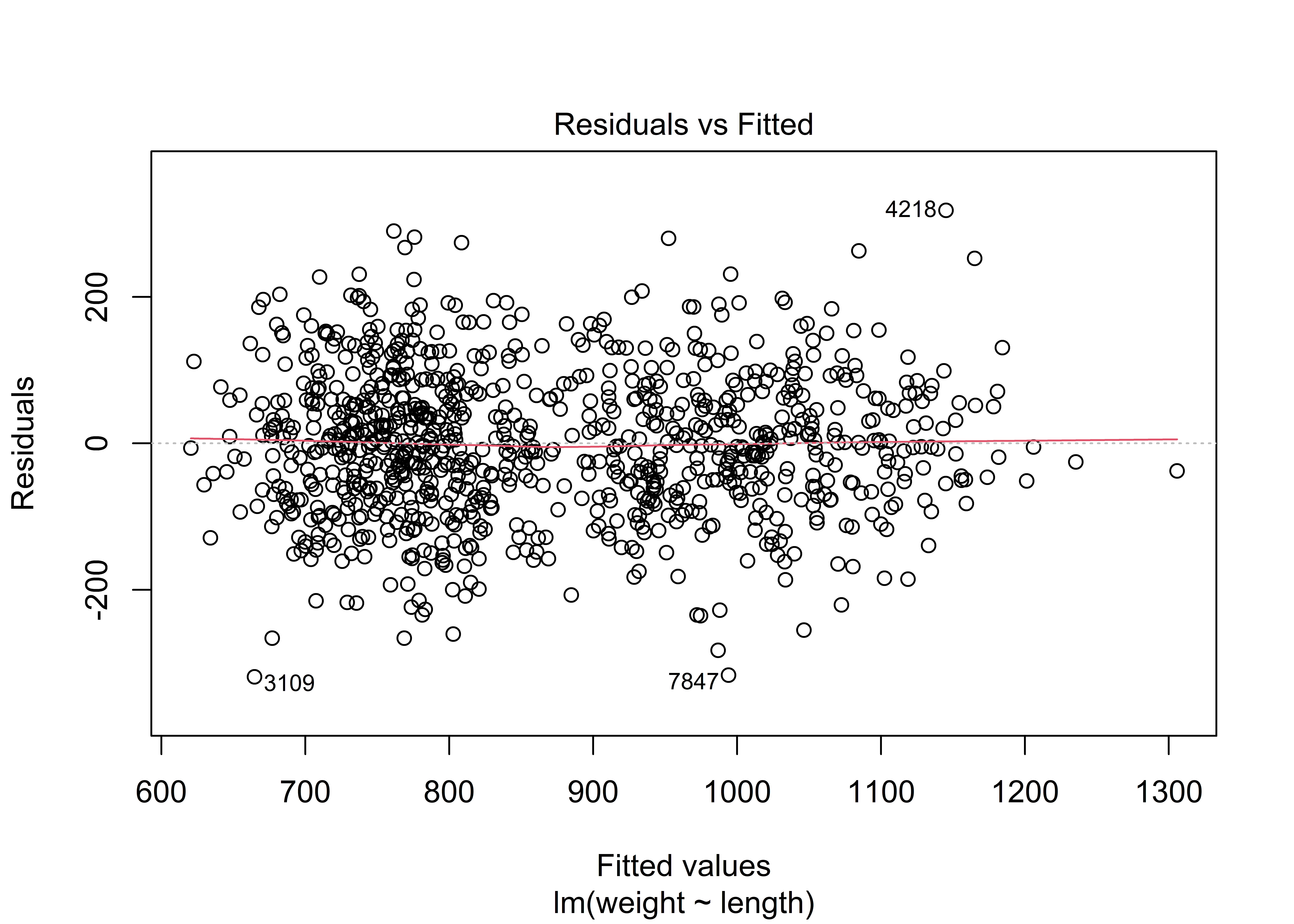
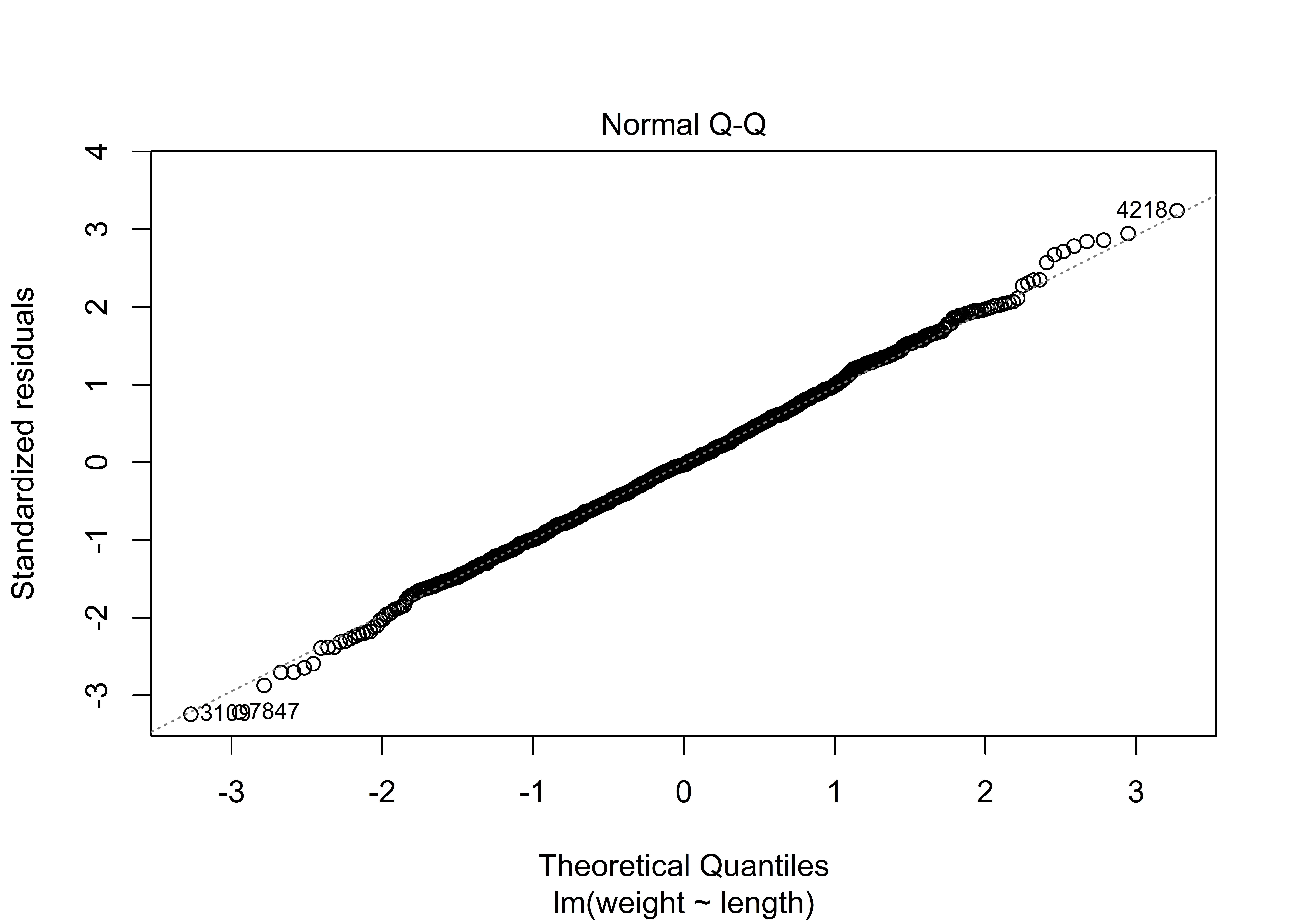
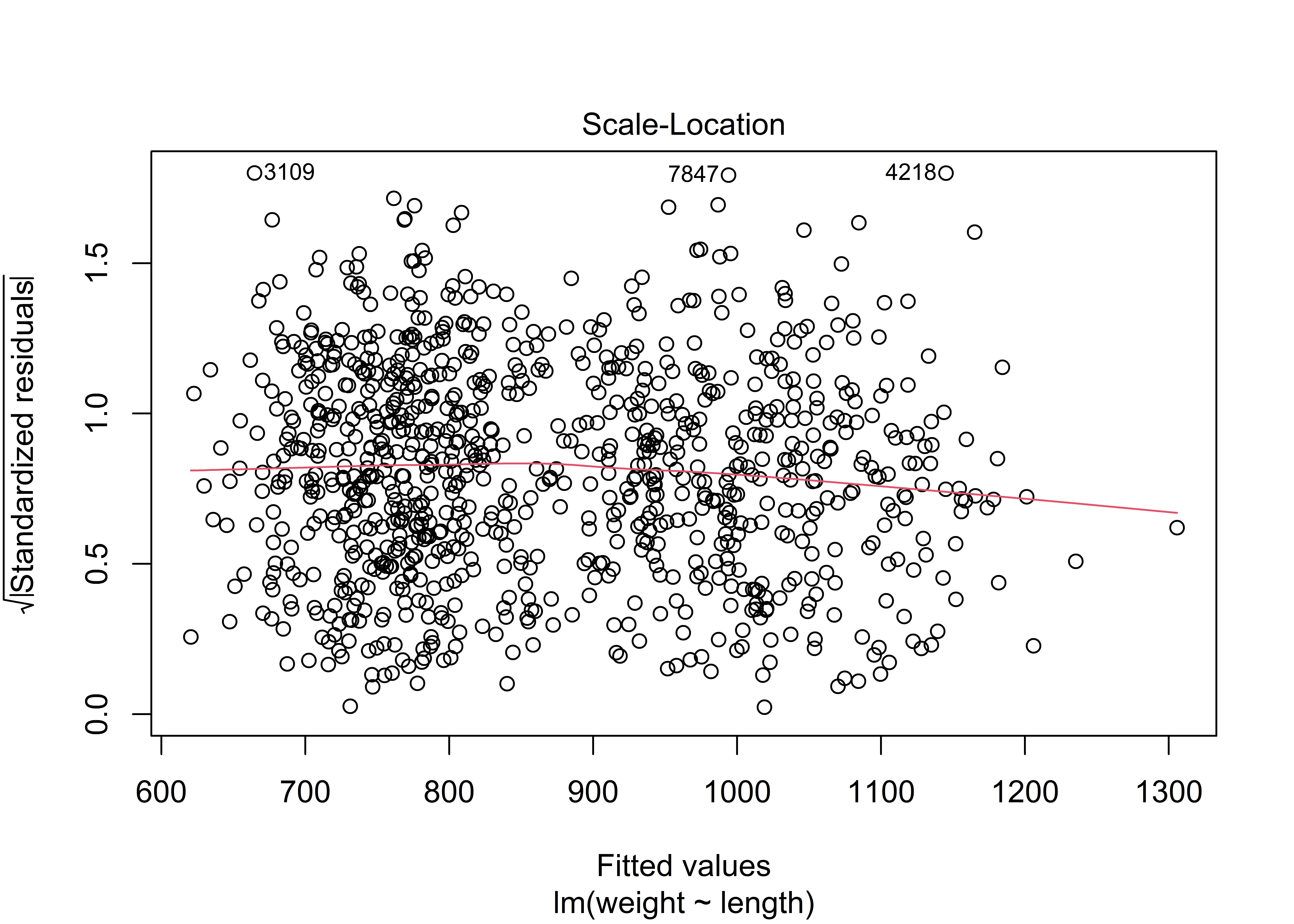
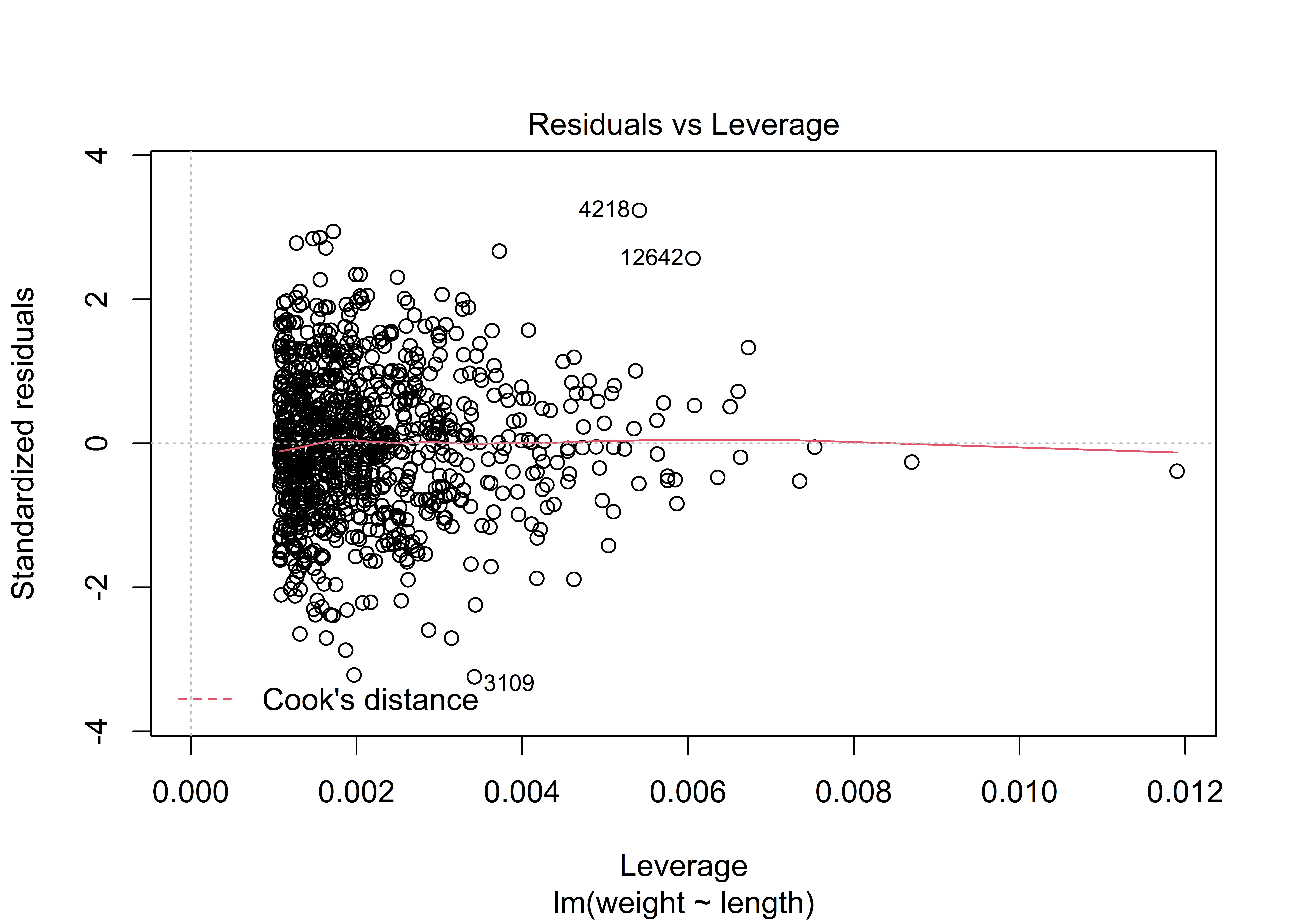
Hmmm. You may have expected to see a graph of the linear relationship itself. But no. This function returns a series of plots that are intended to be used for diagnostic testing.
Let’s try one more method. If we have a new Tauntaun whose weight is, say 350 meters, we could use these coefficients to predict it’s weight: intercept + 350 * length = r round(int * 350 * slope,2)weight units.
By default, the only pieces of information included in the output are estimates for the coefficients (for both the intercept and Tauntaun length). It’s worth repeating: Much more information is out there, but you have to ask for it! As with the other statistical tests we examined, the result of the regression model is a list with a complicated structure, which you can see by using the str function. Then, you can extract the pieces you need using an extraction method such as [[ ]] of $. Alternatively, methods may exist for extracting pieces of the output for you.
9.6 Another Pep Talk
Way to go! That ends our short introduction to statistical functions in R. Statistical analysis is R’s bread and butter, and our goal here was to introduce you to a basic process to work through a statistical test in R. Regardless of which function you use, remember these steps:
- Identify the function needed.
- Read the help page.
- Execute the examples in the help page with the example function.
- Save the result as an object in R.
- Use the
summaryandstrfunction on the sample output so that you can determine what sort of object the analysis returns. - Use
methodsto check for functions that work on your returned object.
At this point, we hope you are maintaining a positive demeanoR. Practice really does make perfect and the most important thing is that you know how to help yourself when you get stuck.
In this chapter we talked about working through the statistical test help files, understanding the structure of your data inputs and test outputs, and interpreting the test results. You can generalize this process to work through most problems in R. And remember, R’s strength is in its open-source community. There are lots of good online resources that can get you out of an R bind. Here are a few:
If you are new to statistics, a few free courses may be of interest:
Hang in there and see you in next chapter, where we finally have enough background to start writing our Annual Tautaun Harvest Report in RMarkdown.