Chapter 7 Data Wrangling - Part 2
Packages Required:

* rgdal - a package for working with spatial data
7.1 Introduction
Welcome back, data wrangler. In this chapter, we’ll continue building our R function vocabulary, and practice with sorting, merging, and plotting data. This chapter builds on Chapter 6, where we created harvest_clean.Rdata, a file that is cleaned of data entry errors, and hunter_clean.RData file:
- harvest_clean.RData
- hunter_clean.RData
Remember that our ultimate goal is to write an annual report to the US Fish and Wildlife Service that summarizes the harvest by age, sex, date, town, and other variables. Our mission now is to combine these two datasets into one, and also merge in the spatial dataset we downloaded from the web. In the process, we’ll also learn how to remove observations and columns, add observations and columns, and sort the data. We’ll also spend time with a few more plotting functions with both base R plotting functions and with ggplot2.
All of this hard work will help us create our annual report in RMarkdown, which we’ll done in a later chapter.
For this chapter, create a new script and name it chapter7.R.
Before we begin, let’s confirm both data files are located in your datasets folder:
## [1] TRUE## [1] TRUEYou might recall that the harvest_clean.Rdata file contains records of all the Tauntauns that have been harvested, while the second contains records of hunter information. Both datasets share a common column, hunter.id, which identifies who harvested which animal.
We can begin reading in these files and refreshing our memory about what information each file contains. We already know the read.csv function, but what function will read in the .Rdata file? For that, we use the load function.
# read in the file and store it as an object called harvest
load(file = "datasets/harvest_clean.RData")

# look at the structure, notice it is a data frame, and look for the hunter.id column
str(harvest)
## 'data.frame': 13351 obs. of 16 variables:
## $ hunter.id : int 285 56 549 296 521 355 674 297 7 388 ...
## $ age : int 1 1 1 1 1 1 1 1 1 1 ...
## $ sex : Factor w/ 2 levels "f","m": 1 1 1 1 1 1 1 1 1 1 ...
## $ individual : int 1 2 3 4 5 6 7 8 9 10 ...
## $ species : chr "Tauntaun" "Tauntaun" "Tauntaun" "Tauntaun" ...
## $ date : Date, format: "1901-10-08" "1901-11-13" "1901-12-26" "1901-12-11" ...
## $ town : Factor w/ 255 levels "ADDISON","ALBANY",..: 196 10 92 192 241 152 8 202 136 32 ...
## $ length : num 277 312 275 267 272 ...
## $ weight : num 699 718 551 700 613 ...
## $ method : Factor w/ 3 levels "bow","lightsaber",..: 2 3 1 3 1 2 2 1 2 2 ...
## $ color : Factor w/ 2 levels "White","Gray": 1 2 1 2 2 2 1 2 1 1 ...
## $ fur : Ord.factor w/ 3 levels "Short"<"Medium"<..: 3 3 3 3 3 1 1 3 2 3 ...
## $ month : num 10 11 12 12 11 10 11 10 11 12 ...
## $ year : num 1901 1901 1901 1901 1901 ...
## $ julian : num 281 317 360 345 325 291 308 277 322 348 ...
## $ day.of.season: num 8 44 87 72 52 18 35 4 49 75 ...Incidentally, in RStudio you can invoke the load function by double-clicking on the .RData file.
Do you see the object harvest_clean in your global environment? We don’t. Instead, we see a new object called harvest. This was the name of the object that we saved as the .Rdata file in the last chapter. Notice that it is a data frame. We can expect the same behavior when we load hunter_clean.RData - the objects within an .RData file are named at the time the .RData file was created with the save function. Our two .RData files contain only a single object, but .RData files can contain multiple objects.
# read in the file and store it as an object called hunter
load(file = "datasets/hunter_clean.RData")

# look at the structure, notice it is a data frame, and look for the hunter.id column
str(hunter)
## 'data.frame': 700 obs. of 3 variables:
## $ hunter.id : int 1 2 3 4 5 6 7 8 9 10 ...
## $ sex.hunter: Factor w/ 2 levels "f","m": 2 2 2 2 2 1 2 2 2 2 ...
## $ resident : logi TRUE FALSE TRUE TRUE FALSE TRUE ...Don’t forget to look for these new objects in your global environment!
7.2 The ‘merge’ Function
Notice that both datasets have a column called hunter.id, which is the unique number that identifies each hunter. It would be useful to merge these two data frames into one, and we’ll do that with the merge function.
Before we use R to merge, let’s talk a bit about merge types from a database point of view. Suppose we have two mini-datasets that we need to merge: the first contains a few harvest records while the second contains hunter records. Hold out your hands, and pretend your left hand is holding the harvest dataset, and your right hand is holding the hunter dataset. Let’s call the left hand table (harvest) x, and the right hand table (hunter) y.
When merging two tables, there are options for which records to keep in the final, merged table. These options are called “join types” in the database world. There are several different join types, but four commonly used types are 1) inner join, 2) outer join, 3) left join, and 4) right join. Let’s look at how these differ. In the figure below, the merge type is shown in red, and, as a sneak preview, the R code is shown in blue.
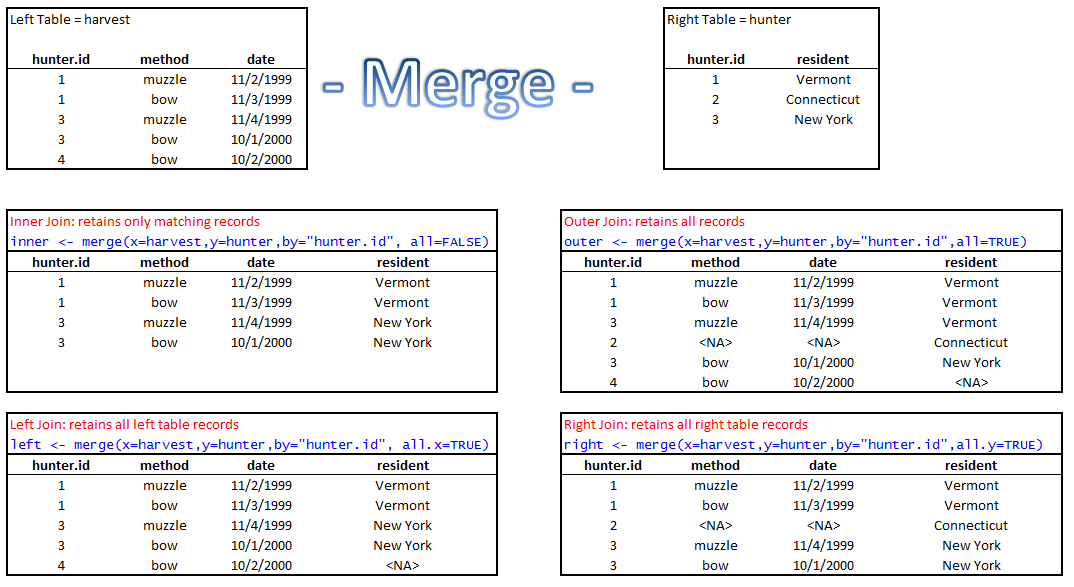
Figure 7.1: Different merging options.
If our left hand table is harvest, and our right hand table is hunter, then the result of an “inner join” (upper left example) would be a table that includes only those rows where there was a complete match (the intersection). Remember that we are joining on the columns, hunter.id. In this case, only records for hunter.id’s 1 and 3 are retained because those are the only records present in both datasets.
An “outer join” (upper right example) would be a table that includes all records from both harvest and hunter, even if there is not a match on the linking field. The missing values would be populated with NA or <NA>, depending on the datatype.
A “left join” (lower left example) would keep all records in the left table, and only those records in the right table where there is a match in the left table. Again, any missing values are populated with NA. A “right join” (lower right example) would keep all records in the right table, and only those records in the left table where there is a match in the right table.
R’s merge function does not use the “join” syntax, although it is similar in spirit.
Take a look at the merge helpfile, and you’ll see several arguments of note. The arguments appear if you use your tab key immediately after the first parenthesis.
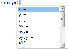
Figure 7.2: The merge argument prompt.
The first two arguments specify x and y. These are the two tables to merge on. Pay attention to what you call x (analogous to a “left table” in database lingo such as SQL) and y (analogous to a “right table” in SQL). The arguments by, by.x, and by.y point to which column to merge on. In our case, it is hunter.id, which is common to both data frames, and each table has this exact same column name, so we can just use by. (If the columns names were different between the two tables, you would need to specify by.x and by.y to tell R which columns to merge on.)
After the by arguments, you’ll see several arguments that begin with the word all. This is where you specify the join type:
- all.x - logical, keeps all records from the table x (similar to a left join). The default is FALSE.
- all.y - logical, keeps all records from the table y (similar to a right join). The default is FALSE.
- all - logical. FALSE will give an inner join, while TRUE will give an outer join.
Sometimes the merge types are visualized with a Venn diagram, as in this image borrowed from the book, R for Dummies.
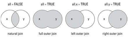
Figure 7.3: The merge Venn diagram.
Before we consider the merge type, it may be useful to know which id’s are present in both datasets, and if any that are present in the harvest dataset are missing from the hunter dataset, and vice versa.
Let’s do that now, using the unique function:
# return a vector of unique entries for hunter.id from the hunter data frame
unique.hunter  <- unique(hunter$hunter.id)
# obtain the sample size with the length function
length(unique.hunter)
## [1] 700So, there are 700 unique hunter.id’s in our hunter data frame. How about the harvest data frame?
# return a vector of unique entries for hunter.id from the harvest data frame
unique.harvest  <- unique(harvest$hunter.id)
# obtain the sample size with the length function
length(unique.harvest)
## [1] 700OK, so now we know that 700 hunters are in the hunters data frame. This means that every hunter actually got a Tauntaun at some point or other.
Suppose we wanted to know if hunter #17 is in the hunter dataset. To determine this, we can use either the %in% operator or the match function . . . both do the same thing, but return different results: %in% will return TRUE or FALSE, whereas match will return the position. These are both very, very useful functions.
For example, to ask if hunter.id 17 is in the unique.hunter vector, we would use this notation:
## [1] TRUETo get the actual position of this record, we would use match or which:
## [1] 17## [1] 17This tells us that hunter.id 17 is the 17th element in the unique.hunter vector.
Suppose our neighbors purchased Tauntaun hunting license, and they have id numbers 543 and 902. We could inquire as to whether they appear in unique.harvest . . . this will return TRUE or FALSE for each entry.
## [1] TRUE FALSESomehow neighbor 902 is not present in the hunter dataset. Perhaps this new license sale has not been logged yet.
Let’s find out how many Tauntauns neighbor 543 harvested.
## [1] 1122 1468 3351 4357 4359 4619 4652 6101 8082 10177 10285 10606 11371 12988 13097Remember, the which function will return the indices (positions) where the result evaluates to TRUE. In this case, row 1122 in the harvest dataset is the first harvest record for hunter 543. Let’s peek at his kills using dataframe subsetting [r,c]. Here, the rows we wish to inspect are those provided by our indices, and we will look at all columns 1:7.
##       hunter.id age sex individual  species       date         town
## 1122        543   1   f       1122 Tauntaun 1902-12-18          JAY
## 1468        543   2   f       1468 Tauntaun 1902-11-02       GOSHEN
## 3351        543   1   m       3351 Tauntaun 1904-12-27     SANDGATE
## 4357        543   1   f       4357 Tauntaun 1905-10-29      ADDISON
## 4359        543   1   f       4359 Tauntaun 1905-12-28       LOWELL
## 4619        543   1   m       4619 Tauntaun 1905-11-11       CANAAN
## 4652        543   1   m       4652 Tauntaun 1905-10-16         EDEN
## 6101        543   1   m       6101 Tauntaun 1906-12-24   CHITTENDEN
## 8082        543   3   f       8082 Tauntaun 1907-11-03   BURLINGTON
## 10177       543   1   f      10177 Tauntaun 1909-11-14      ADDISON
## 10285       543   1   f      10285 Tauntaun 1909-11-27       ATHENS
## 10606       543   1   m      10606 Tauntaun 1909-12-19    HYDE PARK
## 11371       543   3   m      11371 Tauntaun 1909-11-12   NORTH HERO
## 12988       543   3   m      12988 Tauntaun 1910-10-18 WEST WINDSOR
## 13097       543   3   m      13097 Tauntaun 1910-11-29        ESSEX
Let’s now merge the harvest data (harvest) with the hunter data (hunter), where harvest will be x and hunter will be y. Can you think of what merge type to use? We’ll use the left join so that we retain all harvest records.
# merge the data frames by the column hunter id with a full outer join.
harvest <- merge(x = harvest, y = hunter, by = "hunter.id", all.x = TRUE)

# now look again at dataset names
names(harvest)
## [1] "hunter.id" "age" "sex" "individual" "species" "date" "town" "length" "weight"
## [10] "method" "color" "fur" "month" "year" "julian" "day.of.season" "sex.hunter" "resident"## hunter.id age sex individual species date town length weight method color fur month year julian day.of.season sex.hunter
## 1 1 1 m 411 Tauntaun 1901-10-24 CANAAN 384.22 1083.0890 lightsaber Gray Long 10 1901 297 24 m
## 2 1 1 m 3224 Tauntaun 1904-10-06 ELMORE 301.63 607.3689 lightsaber Gray Short 10 1904 280 6 m
## 3 1 1 f 212 Tauntaun 1901-11-18 MILTON 282.61 864.6539 lightsaber Gray Short 11 1901 322 49 m
## 4 1 2 m 7896 Tauntaun 1907-12-23 GLASTENBURY 399.50 855.1852 muzzle Gray Short 12 1907 357 84 m
## 5 1 1 m 12322 Tauntaun 1910-10-15 STRATTON 406.67 1061.7292 muzzle White Medium 10 1910 288 15 m
## 6 1 1 f 51 Tauntaun 1901-11-29 SANDGATE 290.65 867.9066 lightsaber Gray Short 11 1901 333 60 m
## resident
## 1 TRUE
## 2 TRUE
## 3 TRUE
## 4 TRUE
## 5 TRUE
## 6 TRUEMerging is one of those activities you’ll undoubtedly use often when working with data frames. But there are other ways to merge data in R. For example, as we’ll soon see, you can add rows and columns to a dataset, and for this R’s cbind and rbind functions do the work:
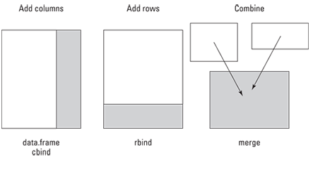
Figure 7.4: Use cbind and rbind to add rows and columns to a dataframe.
7.3 The rbind Function
Our data looks pretty good now, so – wait – what’s that? After all this processing, you were just handed an additional record that was not included in the data? No worries! We’ll show you how to add it your nice, clean dataset. Let’s have a look:
- hunter.id: 24
- age: 3
- sex: f
- individual: 7498
- species: tauntaun
- date: 1978-10-02
- town: MONTPELIER
- length: 10
- weight: 40.3
- method: bow
- color: Gray
- fur: Short
Don’t forget that you’ll now need to enter month, julian, and day.of.harvest as well, along with hunter information. Let’s add the record to the harvest object, right here in R.
The data.frame function can be used to create an object which we will call newRecord. We can’t use the c function because that will create a vector, and if you recall, vectors store only one datatype. Notice the use of indentation in the following code to keep it readable:
# use the data.frame function to create a new data frame with just one record
newRecord <- data.frame(hunter.id = 24,
                       age = 3,
                       sex = "f",
                       individual = 7498,
                       species = "Tauntaun",
                       date = as.Date("1978-10-02"),
                       town = as.factor("MONTPELIER"),
                       length = 336,
                       weight = 850,
                       method = as.factor("bow"),
                       color = as.factor("Gray"),
                       fur = as.factor("Short"),
                       month = 10,
                       year = 1910,
                       julian = 276,
                       day.of.season = 2,
                       sex.hunter = as.factor('m'),
                       resident = as.logical("TRUE")
                       )

# look at its structure
str(newRecord)
## 'data.frame': 1 obs. of 18 variables:
## $ hunter.id : num 24
## $ age : num 3
## $ sex : chr "f"
## $ individual : num 7498
## $ species : chr "Tauntaun"
## $ date : Date, format: "1978-10-02"
## $ town : Factor w/ 1 level "MONTPELIER": 1
## $ length : num 336
## $ weight : num 850
## $ method : Factor w/ 1 level "bow": 1
## $ color : Factor w/ 1 level "Gray": 1
## $ fur : Factor w/ 1 level "Short": 1
## $ month : num 10
## $ year : num 1910
## $ julian : num 276
## $ day.of.season: num 2
## $ sex.hunter : Factor w/ 1 level "m": 1
## $ resident : logi TRUENow we have a new object called newRecord, and you can see that it is a data frame with 1 record. You’ll notice that we played it safe and used several coercion functions (e.g., as.character, as.numeric, as.Date, as.factor, etc) to ensure the datatype matched our harvest data frame.
Now we need to bind our newRecord data frame as a new record (row) to our harvest data frame, making sure that the datatypes we need are retained.
The rbind function was created for this purpose. Look at the rbind helpfile, and you’ll see that it “takes a sequence of vector, matrix or data frames arguments and combine by rows.” The companion is called cbind, which as you can guess binds columns.
Reading a bit further down the helpfile we see “For rbind, column names are taken from the first argument with appropriate names: colnames for a matrix, or names for a vector of length the number of columns of the result.” The number of columns must match in order for rbind to work.
Let’s try it. The first argument is the data frame to bind to, and the second argument is the thing to be bound.
##       hunter.id age sex individual  species       date       town length weight method color   fur month year julian day.of.season sex.hunter
## 13352        24   3   f       7498 Tauntaun 1978-10-02 MONTPELIER    336    850    bow  Gray Short    10 1910    276             2          m
##       resident
## 13352 TRUE## 'data.frame': 13352 obs. of 18 variables:
## $ hunter.id : num 1 1 1 1 1 1 1 1 1 1 ...
## $ age : num 1 1 1 2 1 1 2 1 1 2 ...
## $ sex : Factor w/ 2 levels "f","m": 2 2 1 2 2 1 2 1 1 1 ...
## $ individual : num 411 3224 212 7896 12322 ...
## $ species : chr "Tauntaun" "Tauntaun" "Tauntaun" "Tauntaun" ...
## $ date : Date, format: "1901-10-24" "1904-10-06" "1901-11-18" "1907-12-23" ...
## $ town : Factor w/ 255 levels "ADDISON","ALBANY",..: 42 67 129 80 201 178 190 101 193 205 ...
## $ length : num 384 302 283 400 407 ...
## $ weight : num 1083 607 865 855 1062 ...
## $ method : Factor w/ 3 levels "bow","lightsaber",..: 2 2 2 3 3 2 3 1 2 2 ...
## $ color : Factor w/ 2 levels "White","Gray": 2 2 2 2 1 2 1 1 2 2 ...
## $ fur : Factor w/ 3 levels "Short","Medium",..: 3 1 1 1 2 1 2 3 2 1 ...
## $ month : num 10 10 11 12 10 11 10 10 12 10 ...
## $ year : num 1901 1904 1901 1907 1910 ...
## $ julian : num 297 280 322 357 288 333 281 303 355 288 ...
## $ day.of.season: num 24 6 49 84 15 60 8 30 81 14 ...
## $ sex.hunter : Factor w/ 2 levels "f","m": 2 2 2 2 2 2 2 2 2 2 ...
## $ resident : logi TRUE TRUE TRUE TRUE TRUE TRUE ...It looks like rbind merged the data correctly, and our datatypes also look correct. If we misspelled our column names, or if the number of columns did not match, we would get an error.
7.4 The cbind Function
The cbind function works in the same way. The first argument is the data frame to bind to, and the second argument is the thing to be bound. Let’s add a column to the harvest data frame called count, and set all of the values to 1. (Note: we could just use harvest$count <- 1, but we’ll take this opportunity to use the rep function to create a vector of 1’s, then use the as.data.frame function to convert it to a data frame, and then cbind to bind the two.)
First, let’s create an object called count, which will be a vector:
# create a new vector called count, set its value to 1, then convert to a dataframe
count  <- rep(1, times = nrow(harvest))
count <- as.data.frame(count)
Now, let’s bind this to the harvest data frame with cbind. This function will allow us to bind our count data frame to the harvest data frame.
## 'data.frame':	13352 obs. of  19 variables:
##  $ hunter.id    : num  1 1 1 1 1 1 1 1 1 1 ...
##  $ age          : num  1 1 1 2 1 1 2 1 1 2 ...
##  $ sex          : Factor w/ 2 levels "f","m": 2 2 1 2 2 1 2 1 1 1 ...
##  $ individual   : num  411 3224 212 7896 12322 ...
##  $ species      : chr  "Tauntaun" "Tauntaun" "Tauntaun" "Tauntaun" ...
##  $ date         : Date, format: "1901-10-24" "1904-10-06" "1901-11-18" "1907-12-23" ...
##  $ town         : Factor w/ 255 levels "ADDISON","ALBANY",..: 42 67 129 80 201 178 190 101 193 205 ...
##  $ length       : num  384 302 283 400 407 ...
##  $ weight       : num  1083 607 865 855 1062 ...
##  $ method       : Factor w/ 3 levels "bow","lightsaber",..: 2 2 2 3 3 2 3 1 2 2 ...
##  $ color        : Factor w/ 2 levels "White","Gray": 2 2 2 2 1 2 1 1 2 2 ...
##  $ fur          : Factor w/ 3 levels "Short","Medium",..: 3 1 1 1 2 1 2 3 2 1 ...
##  $ month        : num  10 10 11 12 10 11 10 10 12 10 ...
##  $ year         : num  1901 1904 1901 1907 1910 ...
##  $ julian       : num  297 280 322 357 288 333 281 303 355 288 ...
##  $ day.of.season: num  24 6 49 84 15 60 8 30 81 14 ...
##  $ sex.hunter   : Factor w/ 2 levels "f","m": 2 2 2 2 2 2 2 2 2 2 ...
##  $ resident     : logi  TRUE TRUE TRUE TRUE TRUE TRUE ...
##  $ count        : num  1 1 1 1 1 1 1 1 1 1 ...
7.5 Sorting Data Frames
Your dataset is looking great, and is almost ready for some preliminary data analysis (which we’ll do after a nice break). Before we end, let’s re-order the table and sort by date, and then by town. Sorting organizes the output in a structured way….it may help you visualize and interpret your data more easily.
Ordering a data frame is a simple task that can be frustratingly tricky until you’ve seen it once or twice. The tricky part that we will use the function order instead of sort, which may seem counter-intuitive. The order function allows sorting by multiple columns if we wish. With the order function, we enter each additional sort vector as an argument of the function separated by commas. The order function will return a vector of indices in the order you specified. Save sort for sorting vectors.
# order the dataset by date and then by hunter.id
harvest <- harvest[order(harvest[,'date'],harvest[,'town']),]

# preview the table
head(harvest,10)
## hunter.id age sex individual species date town length weight method color fur month year julian day.of.season
## 10600 560 1 f 116 Tauntaun 1901-10-01 ADDISON 294.35 677.1833 lightsaber White Long 10 1901 274 1
## 1658 89 1 f 53 Tauntaun 1901-10-01 BETHEL 315.05 880.4345 bow Gray Long 10 1901 274 1
## 920 49 3 m 822 Tauntaun 1901-10-01 GUILFORD 426.53 1039.2828 muzzle White Medium 10 1901 274 1
## 2018 108 3 f 795 Tauntaun 1901-10-01 HARDWICK 270.19 624.4626 lightsaber Gray Medium 10 1901 274 1
## 4287 225 1 m 468 Tauntaun 1901-10-01 HIGHGATE 448.05 1108.6107 lightsaber White Long 10 1901 274 1
## 12059 633 3 f 809 Tauntaun 1901-10-01 MORGAN 290.53 688.9998 bow Gray Short 10 1901 274 1
## 2765 146 1 m 347 Tauntaun 1901-10-01 NORTON 408.56 995.6644 muzzle Gray Long 10 1901 274 1
## 210 12 1 f 144 Tauntaun 1901-10-01 POMFRET 284.20 662.1701 lightsaber Gray Short 10 1901 274 1
## 11481 602 1 m 384 Tauntaun 1901-10-01 WARREN GORE 360.13 1061.6615 lightsaber Gray Medium 10 1901 274 1
## 8729 462 4 m 902 Tauntaun 1901-10-02 AVERYS GORE 400.07 946.8853 lightsaber Gray Long 10 1901 275 2
## sex.hunter resident count
## 10600 m FALSE 1
## 1658 m TRUE 1
## 920 m TRUE 1
## 2018 m TRUE 1
## 4287 m TRUE 1
## 12059 f TRUE 1
## 2765 m TRUE 1
## 210 m TRUE 1
## 11481 m TRUE 1
## 8729 m TRUE 17.6 Saving the Final Dataset as an .RDS File
Let’s save this file an .RDS file, this time called TauntaunData (to represent the combined hunter and harvest information). Let’s do that now with the saveRDS function:
This will be the file that we will use in future chapters!**
An .RDS file is not the same thing as an .RData file. The saveRDS file is a function that write a single R object to a file. The helpfile title suggests “Serialization Interface for Single Objects”.
Unlike a RData file, an RDS stores a single object in a serialized manner. However, that single object may be a long list of multiple objects. Additionally, R does not retain the original object name as RData files do. (You might recall that the load function is used to read in an RData file, and the names of the objects at the time of their creation are retained). With a single object stored in an RDS file, you can read it in and give it any name you’d like:
# read the TauntaunData.RDS file into R as 'new.data'
new.data <- readRDS(file = 'datasets/TauntaunData.RDS')

# have a peek
head(new.data)
## hunter.id age sex individual species date town length weight method color fur month year julian day.of.season sex.hunter
## 10600 560 1 f 116 Tauntaun 1901-10-01 ADDISON 294.35 677.1833 lightsaber White Long 10 1901 274 1 m
## 1658 89 1 f 53 Tauntaun 1901-10-01 BETHEL 315.05 880.4345 bow Gray Long 10 1901 274 1 m
## 920 49 3 m 822 Tauntaun 1901-10-01 GUILFORD 426.53 1039.2828 muzzle White Medium 10 1901 274 1 m
## 2018 108 3 f 795 Tauntaun 1901-10-01 HARDWICK 270.19 624.4626 lightsaber Gray Medium 10 1901 274 1 m
## 4287 225 1 m 468 Tauntaun 1901-10-01 HIGHGATE 448.05 1108.6107 lightsaber White Long 10 1901 274 1 m
## 12059 633 3 f 809 Tauntaun 1901-10-01 MORGAN 290.53 688.9998 bow Gray Short 10 1901 274 1 f
## resident count
## 10600 FALSE 1
## 1658 TRUE 1
## 920 TRUE 1
## 2018 TRUE 1
## 4287 TRUE 1
## 12059 TRUE 1We’ll be using this file in Chapter 9 and from this point forward.
7.7 Working with Spatial Data
Speaking of towns, your supervisor just walked in and asked if you could display the total Tauntaun harvest by town in a map. Luckily, in Chapter 5 you downloaded a shapefile and placed it in a folder called “towns”. Remember? Let’s look at this file:
## [1] "towns.zip"                     "VT_Data_-_Town_Boundaries.cpg" "VT_Data_-_Town_Boundaries.dbf" "VT_Data_-_Town_Boundaries.prj"
## [5] "VT_Data_-_Town_Boundaries.shp" "VT_Data_-_Town_Boundaries.shx" "VT_Data_-_Town_Boundaries.xml"
A shapefile actually consists of many different files, each holding special information. For example, the attribute table is stored in the dbf file.
Conveniently, there are many excellent R packages for working with spatial information. For example, we can use R to read in the shapefile containing Vermont town boundaries with the package rgdal, which uses the open source Geospatial Data Abstraction Library drivers–hence the name of the package.
If you haven’t already installed rgdal, do so now:
Let’s load the package so we can use its functions.
We can use the readOGR function to read this shapefile into R.
The helpfile for this function states, “The function reads an OGR data source and layer into a suitable Spatial vector object. It can only handle layers with conformable geometry features (not mixtures of points, lines, or polygons in a single layer). It will set the spatial reference system if the layer has such metadata.” Let’s take a look at this function’s arguments:
## function (dsn, layer, verbose = TRUE, p4s = NULL, stringsAsFactors = as.logical(NA),
##     drop_unsupported_fields = FALSE, pointDropZ = FALSE, dropNULLGeometries = TRUE,
##     useC = TRUE, disambiguateFIDs = FALSE, addCommentsToPolygons = TRUE,
##     encoding = NULL, use_iconv = FALSE, swapAxisOrder = FALSE,
##     require_geomType = NULL, integer64 = "no.loss", GDAL1_integer64_policy = FALSE,
##     morphFromESRI = NULL, dumpSRS = FALSE, enforce_xy = NULL)
## NULL
Looking at the helpfile, we see that the argument dsn is “data source name (interpretation varies by driver - for some drivers, dsn is a file name, but may also be a folder)”. Our file is located in a folder called towns. The second argument is layer, defined as “layer name (varies by driver, may be a file name without extension)”. The layer name is VT_Data_-_Town_Boundaries, which is the name of the shapefile itself (no extension needed).
# use the readOGR function to read in the shapefile
towns <- readOGR(dsn = "towns", layer = "VT_Data_-_Town_Boundaries")
## OGR data source with driver: ESRI Shapefile
## Source: "C:\Users\tdonovan\University of Vermont\Spreadsheet Project - General\R Training\Fledglings\towns", layer: "VT_Data_-_Town_Boundaries"
## with 255 features
## It has 8 fields## Formal class 'SpatialPolygonsDataFrame' [package "sp"] with 5 slotsThe object towns is of class SpatialPolygonsDataFrame , which is an S4 object class imported from package sp. Without getting too far out in the weeds, let’s just say that working with S4 objects requires a slightly different extractor than the S3 objects we have been using so far. With S3 objects, we could extract with the brackets [ ] or the list extractor $. S4 objects use the slot extractor @, and may or may not use the brackets depending on whether the package author has defined methods for them.
To see the information available in an R S4 object, we can use getSlots function on the class of the S4 object. To extract a slot, we call it by name after the “@” extractor. Let’s see if we can view a little bit of the data in this shapefile object:
##         data     polygons    plotOrder         bbox  proj4string
## "data.frame"       "list"    "integer"     "matrix"        "CRS"
Here, we can see that this S4 object has 5 objects within it. If you want to see the gory details, you can try the str function and see if you can locate these 5 objects.
# run this code with increased levels if you want to see deep inside the shapefile
str(towns, max.level = 2)
## Formal class 'SpatialPolygonsDataFrame' [package "sp"] with 5 slots
## ..@ data :'data.frame': 255 obs. of 8 variables:
## ..@ polygons :List of 255
## ..@ plotOrder : int [1:255] 243 69 27 214 197 51 25 20 100 200 ...
## ..@ bbox : num [1:2, 1:2] 424789 25212 581554 279798
## .. ..- attr(*, "dimnames")=List of 2
## ..@ proj4string:Formal class 'CRS' [package "sp"] with 1 slotLet’s plot this shapefile so you can see the 255 towns in Vermont:
Cool! And now, let’s look at a few records from the attribute table, which is stored in the data slot.
##   OBJECTID FIPS6  TOWNNAME TOWNNAMEMC CNTY  TOWNGEOID ShapeSTAre ShapeSTLen
## 0        1  9030    CANAAN     Canaan    9 5000911800   86133926   63085.37
## 1        2 11040  FRANKLIN   Franklin   11 5001127100  105502442   42582.92
## 2        3 11015 BERKSHIRE  Berkshire   11 5001105425  108509286   41941.76
## 3        4 11050  HIGHGATE   Highgate   11 5001133025  155573562   57367.84
## 4        5 11060  RICHFORD   Richford   11 5001159125  111897347   42398.62
## 5        6 13005   ALBURGH    Alburgh   13 5001300860  123041223   55791.54
## 6        7  9080    NORTON     Norton    9 5000952750  100482148   43902.68
## 7        8  9005   AVERILL    Averill    9 5000902125   98589185   39794.77
## 8        9 19050   HOLLAND    Holland   19 5001933775  100189636   40818.36
## 9       10 19060       JAY        Jay   19 5001936325   87962933   37738.29
Notice a column called TOWNNAME. Can you imagine a new column here, called total.harvest, which provides the total number of Tauntauns harvested for each town? And perhaps coloring our town map to indicate the harvest level by town? That’s where we are headed.
7.8 Summarizing the Harvest with Aggregate
We can quickly tally the total harvest by town using the aggregate function.
The aggregate function lets you aggregate your data in a number of ways, and there are two ways to use it. In the first method, you specify what exactly you want to aggregate, which variables you want to aggregate over, and which function to use for aggregation. Here, we want to sum the column, count, by town:
total.harvest <- aggregate(harvest$count,
                           by = list(town = harvest$town),
                           FUN = sum)

# check the structure of this new object; note that it is a data frame
str(total.harvest)
## 'data.frame': 255 obs. of 2 variables:
## $ town: Factor w/ 255 levels "ADDISON","ALBANY",..: 1 2 3 4 5 6 7 8 9 10 ...
## $ x : num 59 65 36 54 51 48 58 54 41 47 ...## town x
## 1 ADDISON 59
## 2 ALBANY 65
## 3 ALBURGH 36
## 4 ANDOVER 54
## 5 ARLINGTON 51
## 6 ATHENS 48
## 7 AVERILL 58
## 8 AVERYS GORE 54
## 9 BAKERSFIELD 41
## 10 BALTIMORE 47The main catch in aggregate is that the by argument must be referenced as list.
The second method for using aggregate is to use the formula notation, like this:
total.harvest2 <- aggregate(harvest$count ~ harvest$town, FUN = "sum")

# look at the first 10 records
head(total.harvest2, n = 10)
## harvest$town harvest$count
## 1 ADDISON 59
## 2 ALBANY 65
## 3 ALBURGH 36
## 4 ANDOVER 54
## 5 ARLINGTON 51
## 6 ATHENS 48
## 7 AVERILL 58
## 8 AVERYS GORE 54
## 9 BAKERSFIELD 41
## 10 BALTIMORE 47In this notation, we specify what it is we want to aggregate (the counts) as a function of town, and specify the sum function once more. Either way works!
Now we can use merge to merge our new vector, total.harvest, to the attribute table for our town shapefile:
towns@data <- merge(x = towns@data,
                    y = total.harvest,
                    sort = FALSE,
                    by.x = 'TOWNNAME',
                    by.y = "town",
                    all = TRUE)
In this example, we used the by.x and by.y arguments because the column storing town name in the shapefile is “TOWNNAME”, whereas the column storing town name in total.harvest is “town”. We also used the sort argument in this example (set to FALSE), which is critical for accurate label placement.
Let’s take a look at our merged dataset:
##     TOWNNAME OBJECTID FIPS6 TOWNNAMEMC CNTY  TOWNGEOID ShapeSTAre ShapeSTLen  x
## 1     CANAAN        1  9030     Canaan    9 5000911800   86133926   63085.37 60
## 2   FRANKLIN        2 11040   Franklin   11 5001127100  105502442   42582.92 39
## 3  BERKSHIRE        3 11015  Berkshire   11 5001105425  108509286   41941.76 51
## 4   HIGHGATE        4 11050   Highgate   11 5001133025  155573562   57367.84 57
## 5   RICHFORD        5 11060   Richford   11 5001159125  111897347   42398.62 44
## 6    ALBURGH        6 13005    Alburgh   13 5001300860  123041223   55791.54 36
## 7     NORTON        7  9080     Norton    9 5000952750  100482148   43902.68 52
## 8    AVERILL        8  9005    Averill    9 5000902125   98589185   39794.77 58
## 9    HOLLAND        9 19050    Holland   19 5001933775  100189636   40818.36 56
## 10       JAY       10 19060        Jay   19 5001936325   87962933   37738.29 58
Notice that the town names are in column 1, and the total harvest is named x, which is the 9th column.
7.9 Creating the Tauntaun Harvest Map
To create a nice map showing the total harvest by town, we need to add row names to the attribute table, which we can do so with the row.names function. The rownames will be the names of the towns themselves.
We can also replace the name x with Tauntauns with the names function:
# set the rownames of the towns attribute table to the town names
row.names(towns@data) <- towns@data[,1]

# replace the name "x" with "Tauntauns"
index <- which(names(towns@data) == "x")
names(towns@data)[index] <- "Tauntauns"

# take a quick look
head(towns@data)
## TOWNNAME OBJECTID FIPS6 TOWNNAMEMC CNTY TOWNGEOID ShapeSTAre ShapeSTLen Tauntauns
## CANAAN CANAAN 1 9030 Canaan 9 5000911800 86133926 63085.37 60
## FRANKLIN FRANKLIN 2 11040 Franklin 11 5001127100 105502442 42582.92 39
## BERKSHIRE BERKSHIRE 3 11015 Berkshire 11 5001105425 108509286 41941.76 51
## HIGHGATE HIGHGATE 4 11050 Highgate 11 5001133025 155573562 57367.84 57
## RICHFORD RICHFORD 5 11060 Richford 11 5001159125 111897347 42398.62 44
## ALBURGH ALBURGH 6 13005 Alburgh 13 5001300860 123041223 55791.54 36Notice the row names in the far left column. Now, let’s take a moment to look at a few functions that are useful in plotting, the topo.colors function and the rev function, along with the pretty function. Check out the helpfiles for each of these (or just ??palattes).
##  [1] "#4C00FFFF" "#2100FFFF" "#000BFFFF" "#0037FFFF" "#0062FFFF" "#008EFFFF" "#00BAFFFF" "#00E5FFFF" "#00FF4DFF" "#00FF0FFF" "#2EFF00FF" "#6BFF00FF"
## [13] "#A8FF00FF" "#E6FF00FF" "#FFFF00FF" "#FFED24FF" "#FFE247FF" "#FFDC6BFF" "#FFDB8FFF" "#FFE0B3FF"
# we can view them by putting them into a pie chart
pie(rep(1,20), col = topo.colors(n = 20, alpha = 1))
##  [1] "#FFE0B3FF" "#FFDB8FFF" "#FFDC6BFF" "#FFE247FF" "#FFED24FF" "#FFFF00FF" "#E6FF00FF" "#A8FF00FF" "#6BFF00FF" "#2EFF00FF" "#00FF0FFF" "#00FF4DFF"
## [13] "#00E5FFFF" "#00BAFFFF" "#008EFFFF" "#0062FFFF" "#0037FFFF" "#000BFFFF" "#2100FFFF" "#4C00FFFF"
The topo.colors function is just one of R’s color palettes. Other related functions include rainbow, heat.colors, and terrain.colors. The argument alpha can be used to set the color transparency.
These colors will be used in creating our map. For each town, we’d like to color-code it so that its color represents the total numbers of harvested Tauntauns.
The pretty function “Computes a sequence of about n+1 equally spaced ‘round’ values which cover the range of the values in x.” Here, x is our total harvested Tauntauns by town, and we would like to create 4 break-points. It’s useful to first use the summary function to understand the numbers we’ll be plotting:
##    Min. 1st Qu.  Median    Mean 3rd Qu.    Max.
##   31.00   48.00   52.00   52.36   57.00   69.00
This gives us an idea of the range of Tauntauns killed. We might wish to “cut” or “bin” the numbers for plotting.
Now we are ready to use the spplot function to create our map. This function is from the package, sp, which was loaded when you loaded rgdal. Let’s take a look at the helpfile and scan it:
This function is a “plot method for spatial data with attributes.” It’s a great function with a lot of depth, and we’ll refer you to a gallery of examples for more information.
Let’s have a look:
twn <- spplot(obj = towns[9], col.regions = col, main = 'Total Harvest By Town', cuts = 5)

print(twn)
Well, that is a nice map – one we can proudly give our supervisor. Notice that the key has 5 “cuts”, which produces 6 color levels. Maps such as this convey a lot of information in a succinct way.
7.10 Next Steps…
You’ve learned quite a few functions for working with data, both in terms of manipulating the data and plotting it in different ways. We’ve been using many of base R functions in our data wrangling so far. In the next chapter, we’ll introduce you to an R package called dplyr, which was developed for clean data wrangling. See you there.