Chapter 5 Projects
Packages needed:

* readxl
* clipr
Now that you have a general idea of R functions and objects, we can get to the real task at hand as the Tauntaun biologist: analyzing data and preparing an annual report. Up until this point, we have only been working with single files in R - the .R files we created by chapter. However, now that you are going ready to work on analyses for a given topic, like the Tauntaun population analysis, you will be utilizing multiple files, some you’ll create and some that you’ll read in. If you are going to work on analyses for a given topic, like the Tauntaun population analysis, it is wise to start a new RStudio “project”. You can have as many different projects as you’d like, and storing files within a Project will help keep them (and you!) organized.
In this chapter, we’ll be creating a project called Tauntauns that will serve as the basis for all scripts, figures, datasets, etc. used in this primer from this point forward. We will also learn some of R’s functions for working with files, and explore an option for reading in Excel files.
RStudio projects are described in RStudio’s documentation.
From this site we learn that:
When a new project is created, RStudio:
- Creates a project file (with an .Rproj extension) within the project directory. This file contains various project options (discussed below) and can also be used as a shortcut for opening the project directly from the filesystem.
- Creates a hidden directory (named .Rproj.user) where project-specific temporary files (e.g. auto-saved source documents, window-state, etc.) are stored. This directory is also automatically added to .Rbuildignore, .gitignore, etc. if required.
- Loads the project into RStudio and display its name in the Projects toolbar (which is located on the far right side of the main toolbar)
The reference to .Rbuildignore and .gitnore are relevant if you are creating a package or using “code versioning”, which tracks changes made to your script file. This is handy if you ever want to revert back to some previous version, or if you are collaborating with others on a coding project. Click here for a friendly tutorial.
Continuing on with the RStudio project documentation….
When a project is opened within RStudio the following actions are taken:
- The .Rprofile file in the project’s main directory (if any) is sourced by R
- The .RData file in the project’s main directory is loaded (if project options indicate that it should be loaded).
- The .Rhistory file in the project’s main directory is loaded into the RStudio History pane (and used for Console Up/Down arrow command history).
- The current working directory is set to the project directory.
- Previously edited source documents are restored into editor tabs
- Other RStudio settings (e.g. active tabs, splitter positions, etc.) are restored to where they were the last time the project was closed.
When you are within a project and choose to either quit, close the project, or open another project the following actions are taken:
- .RData and/or .Rhistory are written to the project directory (if current options indicate they should be)
- The list of open source documents is saved (so it can be restored next time the project is opened)
- Other RStudio settings (as described above) are saved.
- The R session is terminated.
These benefits will become clear as we build our Tauntaun project. Setting up your work as projects has several benefits:
- If you’re like most people, you’ll likely use R for a variety of purposes, and projects are a natural way to organize your work. You’re basically ready to begin with a single mouse click.
- A project can be used to help organize package materials (which we’ll do in chapter 10).
- A project can be used to make interactive websites via the Shiny web application.
- A project can be used to write a book, such as this one.
5.1 Create the Tauntaun Project
Here, we will create a new Project called Tauntauns. This Project will be used to store all of the materials for our Tauntaun population analysis. Go to File | New Project, click New Directory:
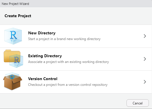
Figure 5.1: The New Project dialogue box.
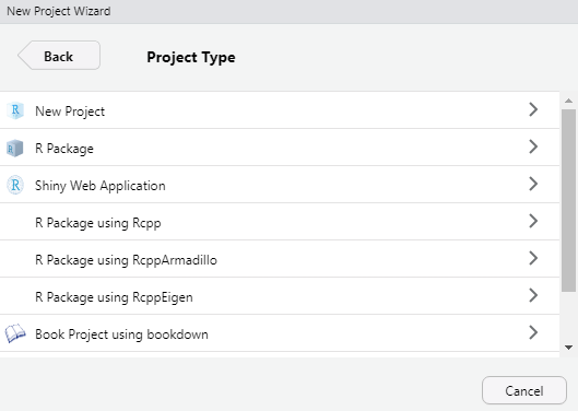
Figure 5.2: Our project will be a new project.
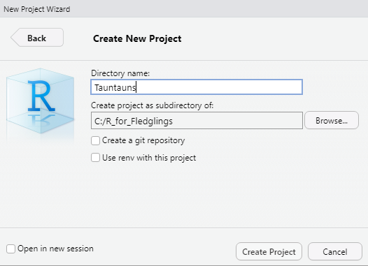
Figure 5.3: Name your project and browse to its location.
RStudio will set things in motion as previously described, making your project the new working directory.
5.2 The .Rproj file
When you created the new project, RStudio created a file called Tauntauns.Rproj. Look for this in your RStudio Files tab, and also in your project’s folder.
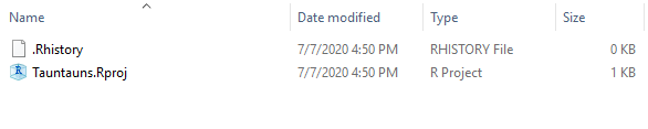
Figure 5.4: Look for the .Rproj file in your new project folder.
RStudio created this file when you created the project, but what does it contain? If you open this in a text editor, you can see that this file stores settings for this project. These settings can be unique for each project, and they override the main settings. Never edit this file directly. You can adjust the project settings by going to Tools | Project Options.
Figure 5.5: Name your project and browse to its location.
For now, the R General tab is of interest to us, which focuses on storage of .RData and history. Remember that an .RData file stores objects in your workspace (global environment), while the .Rhistory file stores your code history. Click on each drop-down to see what options are available to you.
Behind the scenes, these options invoke several R functions, including:
save.imagesavehistoryloadloadhistory
The global settings are the default settings for a project, so if the global settings suit you, you don’t need to change a thing. We learned about the global options back in Chapter 2: you can find them by going to Tools | Global Options.
Figure 5.6: If you do not change project options, R will use the default options provided in the global options tab.
If you are working on a project that involves objects that have taken considerable time to create, you may wish to save your work to the .RData file for that project. When the project is reopened, you have the option of loading these objects back into the global environment automatically. This is totally up to you.
Close out of RStudio, and now, using your computer’s file browser, navigate to and double click on Tauntaun.Rproj file. When you click on a project file, RStudio opens and sets several things in motion. It selects the Files tab in the lower right pane so that you can see all of the files associated with the project, and sets this directory as the working directory, and loads the workspace if instructed to do so. We don’t have any scripts or workspace items yet, so your screen will look like something shown below. The blank script shown in the script editor is the result of going to File | New File | R Script, which brings up a new script called Untitled1. In the Files tab, notice that an empty .Rhistory file has been created (since our default option to Always save history has been checked).
Figure 5.7: Your new project will look fairly bare.
5.3 File Management in R
Our project is currently devoid of any folders, R scripts, or other files. We’ll take some time now to create the directories and download the files that you’ll need for future chapters. This will give us an opportunity to introduce several of R’s file management functions. We will be downloading two CSV files, one shapefile, and one Excel file from the web, and placing them in folders in our Tautaun project. For the rest of this chapter, you can either enter your code into the console and submit commands there, or you can type the commands into the new R script (save this script as chapter5.R).
5.3.1 File paths
A file path specifies the location of a file on your computer or on the web. In the next sections, we’ll be downloading files that we need for future chapters, and storing them on your computer. Because we need to know where to store these files and how to retrieve them, it’s critical that you understand the concept of a file path.
File paths can be absolute or relative paths.
An absolute file path contains your computer’s root directory and all other subdirectories that contain a file or folder. In Windows the root directory is usually the C drive; in linux and MacOS it begins with a forward slash / or tilde ~.
A relative file path locates your file relative to your working directory, which should be your Tauntaun project directory (one of the benefits of using projects is that the working directory is automatically set upon opening).
It’s useful to verify this:
[1] "C:/R_For_Fledglings/Tauntauns/"R returned the absolute file path (we’re on a Windows machine). We interpret this path to mean that we start in the C drive, drop down to the folder called “R_For_Fledglings”, then drop to the folder called “Tauntauns”. Notice that R uses only forward slashes in a file path regardless of the operating system. Never forget this! Also note that the file path is enclosed with quotes.
If you are a Mac or Linux user, your path might look like this:
[1] "/Users/[username]/R_For_Fledglings/Tauntauns"

or

[1] "~ R_For_Fledglings/Tauntauns/"
Why all this fuss over forward versus backward slashes? In computing, the backslash has a special function, which is to escape (or cancel) the special meaning of the next character. The backslash key is located above the Enter key. If we accidentally use the backslash in a file path, R may or may not recognize the following character as a special character to escape, but the intended command will not be completed whether it produces an error or not. For example:
# R interprets the backslash as an escape function, so the "R" character
# in R_for_Fledlgings has no special meaning-- this will return an error

dir("C:\R_For_Fledglings\Tauntauns\")
Error: '\R' is an unrecognized escape in character string starting ""C:\R"Of course, you can navigate via the Files tab in RStudio to see what’s there.
We can peer into the Tauntauns folder with the dir function, specifying the absolute file path.
[1] "Tauntauns.Rproj"You should see the .Rproj file. By setting the argument all.files to FALSE, only the visible files are returned (try it again with all.files = TRUE).
If you don’t know the absolute file path for a given file, don’t forget that the choose.dir or tk_choose.dir functions can be used to interactively select a file or folder on your machine . . . R will return the absolute file path in the console.
We could also peer into the Tauntauns folder by specifying the relative file path. We can see that R is calling our Tauntauns folder the working directory. If we now use the dir function and pass no arguments to it, R will return the files within the working directory.
[1] "Tauntauns.Rproj"Notice that R returned a list of files (well, one) within the directory specified (our working directory) . . . the full file path is not given.
We’ll practice with absolute and relative file paths shortly.
Our goal is to now create 3 folders within the Tauntaun project directory that will store files that we need for future chapters. These folders will be called datasets, towns, and simulations.
5.4 The datasets directory
When you started your job as the Tauntaun biologist, your supervisor suggested that you will be working with two datasets for your work. It’s handy to keep our project files organized, so let’s start by creating a new directory (folder) called datasets within our project directory. In RStudio, you can easily create a directory by clicking on the  icon. However, while you can easily do this with menu options, here we will show you how to create a new directory using code. The
 dir.create function will help us with this task:
Next, let’s create the new directory. If the directory already exists, R will indicate so and not overwrite your existing folder.
# create the directory
dir.create(path = "C:/R_for_Fledglings/Tauntauns/datasets")

# check the directory using the absolute file path
dir(path = "C:/R_for_Fledglings/Tauntauns", all.files = FALSE)
[1] "datasets" "Tauntauns.Rproj"If you are on a Mac or Linux, change the file path as needed.
[1] "datasets" "Tauntauns.Rproj"You can see the .Rproj file, along with the datasets folder.
Now, let’s grab some data! Into this datasets directory, let’s copy the two CSV (comma separated values) files that are posted on the R for Fledglings website:
- TauntaunHarvest.csv - this file provides information about Tauntauns that were harvested.
- hunter.csv - this file provides information about Tauntaun hunters.
While you can download these files from the web in your usual way, let’s use some R functions instead.
In the next section of code, we’ll use the shortcut for the help function to learn about the read.csv function, which is the main way R reads a csv file. After you’ve scanned through the helpfile (don’t skip this step), we’ll use this function to read in the two csv files from the web.
Let’s also use the args function to see the arguments directly:
## function (file, header = TRUE, sep = ",", quote = "\"", dec = ".",
##     fill = TRUE, comment.char = "", ...)
## NULL
As you see in the help file, the read.csv function is a convenience wrapper for the function read.table, which means that this function calls read.table, but simplifies things so that some arguments are pre-populated with values pertinent to csv files. As a result, this function has only a few key arguments.
The argument named file is the path to the csv file. We’ll get to this shortly. The argument named header has a default value of TRUE. A header is a column heading. The argument header = TRUE works for us because our csv file has column names stored in row 1. If this is not the case, you would enter header = FALSE. The argument named sep has a default of “,”. This makes sense because a csv file stores data that are separated by commas. There are other arguments as well that have default values set for csv formats.
The last note to observe is that read.csv can be used to read data through a variety of connections, including web addresses. If the csv is located on the web, the file argument would be something along the lines of file = “http://www.somewhere.com/data.csv”. Notice the quotes (since the file argument is expecting a string.)
Our goal is to place the two csv files into the datasets folder. For the first file, we will demonstrate how you can acquire the file using the absolute file path approach. We’ll store the file’s url as an object in R. Then, we’ll use the url function to open the web connection, and nest this within the read.csv function. With this method, we’ll read in the csv file and store it as an R object called harvest, and then use the write.table function to store this file in the datasets folder:
# first, store the web address of the csv file
url.harvest <- 'https://www.uvm.edu/~tdonovan/RforFledglings/data/TauntaunHarvest.csv'

# the function, url,opens a connection to a web browser
help(url)

# use the read.csv function to create a new object called 'harvest';
harvest <- read.csv(file = url(url.harvest))

# write the file permanently to the data folder
write.table(harvest,
            file = "C:/R_for_Fledglings/Tauntauns/datasets/TauntaunHarvest.csv",
            sep = ",")
The second csv file contains hunter information. For this example, we’ll use the download.file function, and use relative path notation datasets/hunter.csv. This tells R to drop one level down from its working directory to a folder called “datasets”, and to write a file called “hunter.csv”. Notice that this approach creates the file on your machine, but it is not an object in R’s global environment.
Ultimately, the choice of obtaining data via the absolute file path or downloading approach is up to you, and will likely vary from project to project.
# use the download.file function to download files from a web server
help(download.file)

# notice that this creates the file on your machine
download.file(url = "https://www.uvm.edu/~tdonovan/RforFledglings/data/hunter.csv",
    destfile = "datasets/hunter.csv", method = "auto")
We can use the file.exists function to see if R can find our files. This function will return TRUE if the target file was located; FALSE indicates R could not find the file. This is done by pointing to the datasets folder first (which is one level down from our working directory), and then pointing to the file within:
# This relative path will be valid in Windows, Linux, and MacOS
file.exists("datasets/TauntaunHarvest.csv")
## [1] TRUE## [1] TRUEGreat! We’ll be working with these files in the next three chapters (Chapters 6-8).
5.5 The towns directory
Our next directory (folder) within the Tauntaun project will be called towns, and it will store a shapefile containing the towns of Vermont. The Vermont Center for Geographic Information hosts Vermont spatial data. We need a shapefile that stores Vermont towns called **VT_Data_-_Town_Boundaries-shp.zip**, which is stored as a .zip file.
First, we’ll create our towns directory:
Next, we’ll use R to download this shapefile, unzip it, and store it within towns. Although we could try the download.file function again to download a zip file, it’s tricky because the arguments may vary depending on your operating system. We are on a Windows machine, and set the mode argument to ‘wb’. If you are a Mac user, try “curl” for this argument.
# use download.file to download the two zipped files
download.file(url = "https://opendata.arcgis.com/datasets/0e4a5d2d58ac40bf87cd8aa950138ae8_39.zip?outSR=%7B%22latestWkid%22%3A32145%2C%22wkid%22%3A32145%7D",
    destfile = "towns/towns.zip",
    method = "auto",
    mode = "wb")
Next, we’ll unzip the file with the unzip function:
If this code doesn’t work for you, use a web browser to locate the shapefile of Vermont towns on the Vermont Center for Geographic Information website (https://geodata.vermont.gov/). It should be listed it under the theme Boundaries. Search for towns, and you should see the link “VT Data - Town Boundaries”. Click on the “Download” dropdown, and choose “Shapefile”. Then move the zipped file to your towns folder and unzip it manually.
Let’s use the list.files function to peak inside the towns folder, and you’ll see that a shapefile is actually several files that provide different information about the spatial object.
## [1] "towns.zip"                     "VT_Data_-_Town_Boundaries.cpg" "VT_Data_-_Town_Boundaries.dbf" "VT_Data_-_Town_Boundaries.prj"
## [5] "VT_Data_-_Town_Boundaries.shp" "VT_Data_-_Town_Boundaries.shx" "VT_Data_-_Town_Boundaries.xml"
Terrific. We will be working with these files in future chapters.
5.6 The simulations directory
Finally, we are going to create a third new directory (called simulations) and download one more data file, an Excel file. This file stores inputs needed to simulate a virtual Tauntaun population. We won’t actually work with these data until Chapter 13, but we might as well get all of our data squared away right now.
First, we’ll create the directory and download the Excel file to the new directory
# this will create a directory within our working directory
dir.create(path = "simulations")

# notice that this creates the file on your machine.
download.file(url = "https://www.uvm.edu/~tdonovan/RforFledglings/data/SimHarvest_2020.xlsx",
    destfile = "simulations/SimHarvest_2020.xlsx",
    method = "auto", mode = "wb")
Now make sure the Excel file called SimHarvest.xlsx is located in your simulations directory in the Tauntaun project.
# check to see if the file exists in the working directory
file.exists("simulations/SimHarvest_2020.xlsx")
## [1] TRUESuper! Now, we’ll take this opportunity to make sure that you are able to read in the file to R, even though you won’t be using it until Chapter 12.
5.7 Reading in the Excel Inputs
Unlike a CSV, file, base R cannot read Excel files. Instead, we will need to load a package designed to do this. In this tutorial, we’ll cover a package option that we hope will cover most users: readxl. In addition, we’ll show you how to copy Excel data to the clipboard and save it as an R object. This will be done with the package clipr.
First, if you haven’t installed readxl yet, do so now. Let’s load it, and then scan at the package helpfiles (which are really helpful, have a look at the vignettes as well). The package is part of the tidyverse, described as “an opinionated collection of R packages designed for data science. All packages share an underlying design philosophy, grammar, and data structures.” We will work with a few other tidyverse packages later in the book.
The data on the Excel file are stored in two regions within a sheet called “popmodel”. Let’s review these regions in the spreadsheet. The first region provides the starting population size of Tauntauns by age (0 through 5) and sex. For example, at the beginning of the simulation, there will be 3000 0-year-old females and 1200 0-year-old males.
Figure 5.8: The Tauntaun population seed data.
The second set of inputs is located in cells J2:P7, and these store “vital rates” by age. These are rates that drive the Tauntaun life cycle, such as birth, survival, and harvest rates.
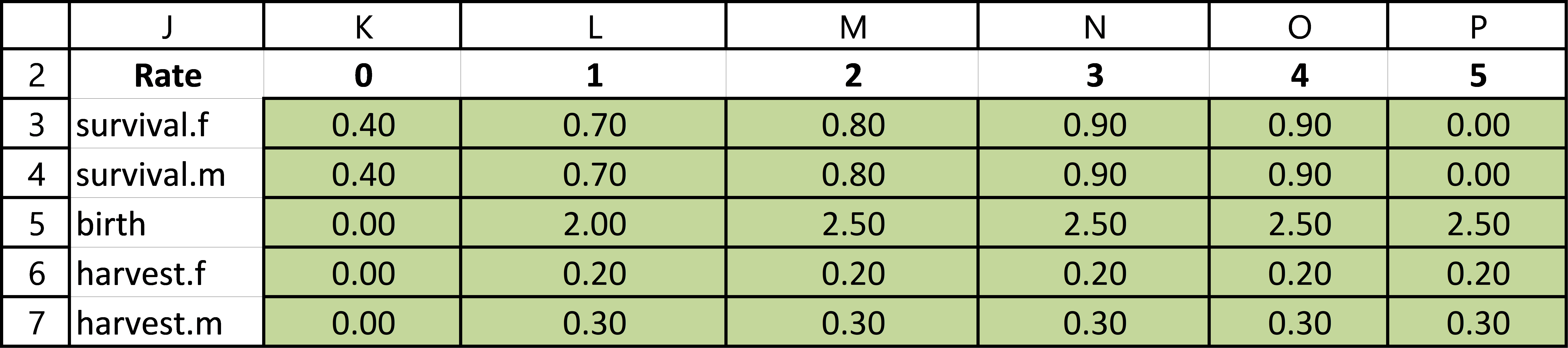
Figure 5.9: Parameters that drive the Tauntaun life cycle.
We’ll call in both sections now, and combine them into a single list called “inputs”. The main function we need is called read_excel. We simply point to the file and identify the range for each of our four inputs.
# read in the section named inputs1
pop.seed <- read_excel(path = "simulations/SimHarvest_2020.xlsx",
                       sheet = "popmodel",
                       range = "A2:G4")

# read in the section named inputs2
pop.params <- read_excel(path = "simulations/SimHarvest_2020.xlsx",
                         sheet = "popmodel",
                         range = "J2:P7")
Let’s have a look at the structure of one of our new objects.
## tibble [2 x 7] (S3: tbl_df/tbl/data.frame)
##  $ Sex: chr [1:2] "females" "males"
##  $ 0  : num [1:2] 3000 1200
##  $ 1  : num [1:2] 1500 900
##  $ 2  : num [1:2] 500 300
##  $ 3  : num [1:2] 300 180
##  $ 4  : num [1:2] 100 60
##  $ 5  : num [1:2] 50 30
Notice that this object is a “tibble”, which is similar to a data frame. Tibbles are part of the tidyverse world, where the tibble package author (Hadley Wickham) describes it in this way: “A tibble, or tbl_df, is a modern reimagining of the data.frame, keeping what time has proven to be effective, and throwing out what is not. Tibbles are data.frames that are lazy and surly: they do less (i.e. they don’t change variable names or types, and don’t do partial matching) and complain more (e.g. when a variable does not exist). This forces you to confront problems earlier, typically leading to cleaner, more expressive code.”
This particular tibble is 2 rows and 7 columns. You should be able to view it in spreadsheet like view by pressing its associated grid button in the global environment. Soon, we will be converting it to a plain-old dataframe.
5.8 Reading Data from the Clipboard
Another option for reading in the Excel data is to use your clipboard. The package clipr can be used read and write from the system clipboard, regardless of what operating system you use.
If you have the file “SimHarvest.xlsx” open, just highlight cells A1:Q2 and copy them, then use the following:
Have a look at the structure of seed. It is a dataframe, not a tibble. You can follow suite for the next input if you wish.
5.9 Saving Inputs as an RData file
Regardless of which approach you have used, you should end up with four objects in your global environment called pop.seed, pop.params. Our goal now is to put these into in a list, turn each portion of the list to a dataframe, and then save the list as an .RData file. In Chapter 12, we can then just call in this file with the load function.
First, let’s use the list function to put these four objects into a list, assigning a name to each section of the list.
# put all inputs into a list called inputs
inputs <- list(pop.seed = pop.seed, pop.params = pop.params)

# look at the structure of the list called inputs
str(inputs)
## List of 2
## $ pop.seed : tibble [2 x 7] (S3: tbl_df/tbl/data.frame)
## ..$ Sex: chr [1:2] "females" "males"
## ..$ 0 : num [1:2] 3000 1200
## ..$ 1 : num [1:2] 1500 900
## ..$ 2 : num [1:2] 500 300
## ..$ 3 : num [1:2] 300 180
## ..$ 4 : num [1:2] 100 60
## ..$ 5 : num [1:2] 50 30
## $ pop.params: tibble [5 x 7] (S3: tbl_df/tbl/data.frame)
## ..$ Rate: chr [1:5] "survival.f" "survival.m" "birth" "harvest.f" ...
## ..$ 0 : num [1:5] 4e-01 4e-01 0e+00 1e-21 1e-21
## ..$ 1 : num [1:5] 0.7 0.7 2 0.2 0.3
## ..$ 2 : num [1:5] 0.8 0.8 2.5 0.2 0.3
## ..$ 3 : num [1:5] 0.9 0.9 2.5 0.2 0.3
## ..$ 4 : num [1:5] 0.9 0.9 2.5 0.2 0.3
## ..$ 5 : num [1:5] 0 0 2.5 0.2 0.3Can you see that this is a list of 2 objects? Look for this object in your global environment, and press the magnifying glass to inspect it further. Our list is a named list, which means each part of the list is named: look for $ pop.seed: to find our initial pop.seed object.
Dig a bit deeper into the inputs list structure and you’ll see each column of information within a section is also identified by a $ – this is because a dataframe (and tibble for that matter) is a list of vectors, all of the same length.
Don’t blow past this information. Knowing how R stores your information – and what kind of data it stores information as – is half the battle when coding.
Remember that you can extract a given portion of the list with the [[ ]] or with $, both of which will return the list element in its original class. All three of the options below do the same thing, and will return a tibble (from read_excel):
## # A tibble: 2 x 7
##   Sex       `0`   `1`   `2`   `3`   `4`   `5`
##   <chr>   <dbl> <dbl> <dbl> <dbl> <dbl> <dbl>
## 1 females  3000  1500   500   300   100    50
## 2 males 1200 900 300 180 60 30## # A tibble: 2 x 7
## Sex `0` `1` `2` `3` `4` `5`
## <chr> <dbl> <dbl> <dbl> <dbl> <dbl> <dbl>
## 1 females 3000 1500 500 300 100 50
## 2 males 1200 900 300 180 60 30## # A tibble: 2 x 7
## Sex `0` `1` `2` `3` `4` `5`
## <chr> <dbl> <dbl> <dbl> <dbl> <dbl> <dbl>
## 1 females 3000 1500 500 300 100 50
## 2 males 1200 900 300 180 60 30For this tutorial, it will be useful to store the 2 list elements as a single class (e.g., all dataframes). We’ll do this because some readers may have a list of tibbles, while others might have a list of dataframes. We all need to be on the same page in future chapters, so we’ll convert all elements to dataframes.
Here, we’ll use the apply function to turn each portion of the list to a dataframe with the as.data.frame function.
This is the first time we’ve used one of R’s “apply” functions, so let’s talk about them. The apply functions “apply a function” across each elements of an object, X. There are several “flavors” of this function:
apply- returns a vector or array or list of values obtained by applying a function to margins of an array or matrix.lapply- returns a list of the same length as X, each element of which is the result of applying FUN to the corresponding element of X.sapply- is a user-friendly version and wrapper of lapply by default returning a vector, matrix or, if simplify = “array”, an array if appropriatevapply- is similar to sapply, but has a pre-specified type of return value, so it can be safer (and sometimes faster) to use.
A quick demo of apply and lapply will help show you how this works:
##      [,1] [,2] [,3]
## [1,]    1    3    5
## [2,]    2    4    6
# to each column into a character (MARGIN = 2 means "by column")
(apply.my.matrix <- apply(X = my.matrix, MARGIN = 2, FUN = as.character))## [,1] [,2] [,3]
## [1,] "1" "3" "5"
## [2,] "2" "4" "6"## [1] "matrix" "array"Let’s do the same thing but use lapply instead; this will return a list:
# do the same thing but use lapply instead; this will return a list
(lapply.my.vector  <- lapply(X = my.matrix, MARGIN = 2, FUN = as.character))
## [[1]]
## [1] "1"
##
## [[2]]
## [1] "2"
##
## [[3]]
## [1] "3"
##
## [[4]]
## [1] "4"
##
## [[5]]
## [1] "5"
##
## [[6]]
## [1] "6"The idea here is that you have an R object (a matrix, array, list, etc.), and you want to execute some function over each element in the object. You can see that in both cases, each element in my.matrix was converted to a character by setting FUN = as.character. The difference is that apply returned a matrix, while lapply returned a list.
Which ‘apply’ function you use depends on what your input is, the function you want to use, and how you’d like to store your result.
Let’s use the lapply function to convert each portion of our inputs list into a dataframe. We’ll use lapply because we want R to return a list. First, though, let’s have a look at the arguments.
## function (X, FUN, ...)
## NULL
The arguments of lapply are “X”, the object to work on (in our case, inputs), and “FUN”, the function that you want to run on each element within harvest (in our case, as.data.frame). Don’t forget that inputs itself is a list. So the function will work through each section of the list (the four inputs), and execute the function you specify.
Let’s try it, but save the result as a new object called sim_inputs.
# use the lapply function change the class to dataframe
sim_inputs  <- lapply(X = inputs, FUN = as.data.frame)

# look at the structure of sim_inputs
str(sim_inputs, max.level = 1)
## List of 2
## $ pop.seed :'data.frame': 2 obs. of 7 variables:
## $ pop.params:'data.frame': 5 obs. of 7 variables:Can you see that each element of this list is now a dataframe? This should give you a glimpse of how powerful the ‘apply’ functions can be in terms of efficient coding, especially when working with large and complex suites of data. We’ll use the ‘apply’ functions in future chapters.
We have one last step in this chapter: we need to save our new object as an .Rdata file so we will be ready to use it future chapters. This is easily accomplished with the save function:
# save the object sim_inputs
save(sim_inputs, file = "simulations/sim_inputs.Rdata")

# check that the file exists
file.exists("simulations/sim_inputs.Rdata")
## [1] TRUE5.10 Summary
Well done! In this chapter, we learned about RStudio’s projects and set up our Tauntaun project. We learned several new functions for working with files and directories, learned how to read in files from Excel, and used our first ‘apply’ function. All of this work sets the stage for smooth progress in the chapters to come.
In the next chapter, we’ll begin working with the csv files in the datasets directory, and will create new scripts for analysis and report writing.
Onward!