Chapter 4 Objects

In addition to entering functions in R, you will create and edit “objects”. . . tons of them . . . in all different sizes, shapes, and flavors. This chapter will introduce you to objects in R. Warning! This is a long chapter, and you don’t have to memorize anything. The goal here is to make you realize that there are many kinds of objects and many kinds of datatypes, and that there are a few key functions that can help you know what kind of object you are dealing with. We’ll be working with objects extensively in future chapters…for now, breathe easy and try to keep the big picture in mind.

Open a new R script file and save it as chapter4.R your R_for_Fledglings directory. Use this script for all of this chapter’s work.

In Chapter 3 we used the sqrt function to calculate the square root of a number. That was neat, but it would be nice to save the result for later.

Creating a new object is as easy as typing the object’s name and assigning a value to it. There are multiple ways to assign values to objects in R. As in many computer languages you can use the equal sign (=) as an assignment operator. Copy the following code into your script, and run it.

# take the square root of 100, and assign it to an object called "result"
result = sqrt(100)

Now we have created an object called result. To verify that, we can type the name of the object, and R will print the value stored for it (emphasing that an object has a name and a value):

# look at the object called result
result

## [1] 10

You can replace these two lines of code with one by wrapping the result = sqrt(100) within parentheses. This creates the object “result” and returns the result.

(result = sqrt(100))

## [1] 10

In this book, we won’t be using the = sign to create objects in R. Instead, we’ll be using the more conventional the left-pointing assignment arrow to create our objects, which looks like this <-. The downside is that we have to type twice as many characters (small con), but the upside is that the directionality of the assignment (name <- value) is clear (big pro). You can also a right-pointing assignment arrow to create objects. However, the left-poining arrow is preferred because it allows us to name the object first, then assign any value to it. In this way, object names are always located along the left margin, which makes our code easier to read, especially when it comes to locating objects within the code.

You can easily create this arrow in RStudio by pressing Alt and dash keys simultaneously (Alt+-). More keyboard shortcuts can be found in the Help menu.

result <- sqrt(100)
result

## [1] 10

Now, let’s remove this object from our global environment:

rm(result)

Let’s bring it back to life, this time with the assign function:

# use the assign function to create an object whose name is result and whose value is 10
assign(x = 'result', value = 10)

# look at the object
result

## [1] 10

Thus, <- and = invoke the assign function. You can learn more about assignment operators with this code:

help(`=`)

You can think of an object in R as if it is a shoebox (object) with a name. Here, the name of the shoebox is “result”, and you can imagine that it is holding a scrap of paper with the number 10 on it. You can name your object (shoebox) anything you want (with a few exceptions), and you can store any value in it (with a few exceptions). For instance we could have named it Tintin if we wanted, but that wouldn’t have been very informative. The most important thing when naming an object is to assign a name that describes its contents and that you can remember later. Perhaps we should have named it sqrtResult. Stay clear of giving your objects names that are names of functions or any key words that seem like computer code, like “break”, “else”, “if,”for“,”TRUE“,”FALSE", etc.

Now lets change the value of our object.

(result <-  sqrt(25))

## [1] 5

Now you see that our “shoebox” named result has a different scrap of paper in it that has the value 5. Notice that we have replaced our first result (10) with the new result (5). R does not give a warning that the current value will be overwritten. If you really want to store the first result, you might change the name of the second result to result2.

An object doesn’t have to be a single value. In fact, as we’ll soon see, objects come in many shapes, sizes, and flavors. For example, if we want to create an object called lowNumbers that stores the numbers 1, 2, 3, 5, and 6 as a single group that skips the number 4, we would enter into our console:

# create an object called lowNumbers, and make it a vector with the numbers 1, 2, 3, 5, and 6
lowNumbers  <-  c(1,2,3,5,6)

# look at the object called lowNumbers
lowNumbers

## [1] 1 2 3 5 6

We used the c function (combine function) to combine the numbers 1, 2, 3, 5, and 6 into a new shoebox (object) called lowNumbers, which has a single scrap of paper with the numbers 1, 2, 3, 5, and 6 in that order. If you use spreadsheets, this is analogous to entering the same numbers in cells A1 through A5 and then naming the entire range A1:A5 “lowNumbers”.

In R, we can also assign objects the value of other objects. If we want to add a new object fiveNumbers that has the same value as our object lowNumbers, we would write the declaration as follows:

fiveNumbers  <-  lowNumbers

Now let’s look at both objects:

# display the object called lowNumbers
lowNumbers

## [1] 1 2 3 5 6

# display the object called fiveNumbers
fiveNumbers

## [1] 1 2 3 5 6

To retrieve an object, just type the name of the object and send it to the console. A little trick to save some typing is to use your tab key . . . enter the first letter of the object, then press tab. A small dialogue box will open that displays objects (including functions). Below, we typed in “r”, then pressed “tab”. Do you see the object called result? You may have scroll a bit. Objects that can be selected are color-coded: functions are light blue, objects are coded in pink, packages have purple P, and dataframes look like a tiny grid. If you press tab again, the highlighted word is inserted.

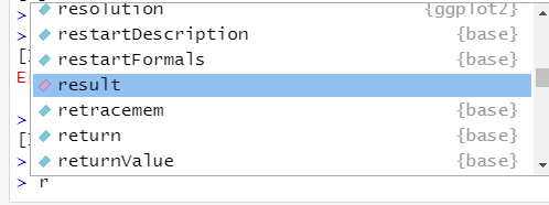
Figure 4.1: The tab key in RStudio is super helpful!

4.1 The Global Environment

Any objects that we create must live somewhere in R. Our objects, fiveNumbers, result, and lowNumbers all live in the global environment. Functions within packages all live in their own package environment.

Although the code below is overkill, it illustrates the fact that objects in R must exist in some environment or other, and that everything that R does is accomplished by a function, even if it happens behind the scenes:

get('result', envir = globalenv())

## [1] 5

In R Studio, click on the Environment tab in the upper right pane, and you’ll see your objects there. You can look at your objects in list view or grid view. Look for this toggle in the upper right hand corner of the Environment Pane, just above the search box: or

Your “list view”" should look something like this:

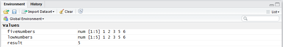
Figure 4.2: The list view.

And the “grid view”" should look something like this:

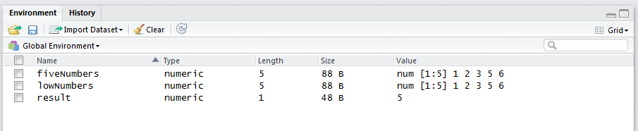
Figure 4.3: The list view.

You can use either view, but the grid view shows more information about your objects, and you can select individual objects. The columns within the grid view include:

Name = name of the object.
Type = type of the object (its mode is shown if the object is a vector; its class is shown if the object is more complicated that a simple vector).
Length = length of the object.
Size = size of the object (in terms of digital information).
Value = current value of the object (what’s in the shoebox).

As we’ll soon see, the column “Type” can be confirmed with the mode function for simple objects (like vectors) or with the class function for more complex objects.

Let’s look at the objects we’ve created in grid view.

We’ve created an object called result, which if you recall, holds the result of the sqrt function we used earlier. The name of this object is result, and it is a number. It’s current value is 5, and R is using 48 bytes of memory to store this number. It has a length of 1 because it stores a single number.

We also created an object called fiveNumbers, which if you recall, is a vector that contains the numbers 1, 2, 3, 5, and 6 in that order. The name of this variable (or object) is fiveNumbers, and the type of information stored in this vector is numeric.

mode(fiveNumbers)

## [1] "numeric"

It has a length of 5 because it stores 5 numbers. R is using 88 bytes to store this object (your result may be a bit different). Under the column “value”, we see num[1:5] 1 2 3 5 6. This is very informative; it tells us that R is storing this object as a vector – a type of object that stores a series of items such as a single row or single column in a spreadsheet. Specifically, the notation [1:5] tips us off that this object is a vector that contains 5 elements (cells). The num notation preceding it indicates that the values stored are numbers (or numeric mode). Then we see the actual values stored within fiveNumbers, which are 1, 2, 3, 5, and 6.

We’ve mentioned that the Environment tab is the Most Valuable Player (MVP) of RStudio. There is no faster way to learn how to code in R than to execute some code, and then look in the Environment pane and see what happened.

4.2 Data Types (Modes)

We now have a few different objects in our global environment, but how exactly does R store them for future use? In this section, we’ll learn about a the most commonly used ‘data types’ or storage modes in R. These include dates, numbers (integers and decimals), and logical (true/false) values.

Let’s create a new vector called fiveRandoms which will be a vector that stores 5 random numbers between 0 and 1, drawn from a uniform distribution. In Excel, this is done by using the RAND function. In R, this function is called runif, which stands for “random uniform”. First, let’s look at the helpfile.

# look at the helpfile
help(runif)

And now we can create our new object.

# create a new object called fiveRandoms, using the runif function
fiveRandoms <- runif(n = 5)

# look at the object called fiveRandoms
fiveRandoms

## [1] 0.6276556 0.4272567 0.9864081 0.6058641 0.5098213

Your random numbers will be different than ours (more on that later).

Now let’s look at the object in the Environment pane. You should see that fiveRandoms also have a numeric type, which is its mode.

Now let’s use the sample function to randomly sample 5 numbers between 1 and 100. It’s important here to look at the helpfile, and to understand each argument.

# look at the helpfile
help(sample)

# look at the arguments for the sample function
args(sample)

## function (x, size, replace = FALSE, prob = NULL) 
## NULL

This function has four arguments: x is a vector you’d like to sample from, size is the number of samples to take, replace indicates whether you’d like to sample with replacement (which means the same numbers can be drawn repeatedly), and prob is used when you want to weight your samples so that some have a higher chance of being selected than others.

Now that you’ve scanned the helpfile and arguments, we can create our object. We’ll draw 5 random samples (with replacement) from a vector containing the numbers 1 through 100. Don’t forget the tab trick for entering function arguments! It should be clear that x, size, replace, and prob are the names of the arguments for the sample function.

# create a new object called fiveIntegers, using the sample function
fiveIntegers  <- sample(x = c(1:100), size = 5, replace = TRUE)

# look at the object called fiveIntegers
fiveIntegers

## [1] 40 76 40 84 64

Now take a look in the Global Environment at this new entry. You should see a new entry under the column Type called integer. Numeric modes include both “integers” and “double”, and RStudio is displaying this more fine-grain information.

If the Environment tab is the MVP of RStudio, the str function is the MVP of R functions for learning about objects.

# look at the structure of the object, fiveRandoms
str(fiveRandoms)

##  num [1:5] 0.628 0.427 0.986 0.606 0.51

# look at the structure of the objects, fiveIntegers
str(fiveIntegers)

##  int [1:5] 40 76 40 84 64

The str function returns the structure of an object in the R console, where it confirms that our object, fiveRandoms is indeed a vector of numbers, and that our object, fiveIntegers, is indeed a vector of integers. Remember that the notation [1:5] indicates that our objects are vectors. We’ll be using the str function repeatedly in this primer.

What about dates? Let’s try it. The function that returns today’s date and time is the date function, with no arguments:

today <- date()
str(today)

##  chr "Wed Jan 06 09:01:05 2021"

What happened here? The object called today is stored as a character (also called a “string” or “text” in other computer languages). The str function indicates this by returning chr, while the word character is displayed in the global environment for this new object. Both suggest the same thing: R is storing the object called today as a string of characters. Objects that are characters can be spotted from afar because the values are in quotes.

Let’s enter the birthday of Nelson Mandela:

birthday  <- 7/18/1918
str(birthday)

##  num 0.000203

Now it is clear that if you want to enter a date into R you have to be careful, or R will think you are using it as a calculator! Here, R returned 7 divided by 18 divided by 1918. You can force the birthday object to be a date by using the as.Date function:

# use the as.Date function to convert Nelson Mandela's birthday to a date
birthday2 <- as.Date("7/18/1918")

Error in charToDate(x) : 
  character string is not in a standard unambiguous format

Hmmmm….R returned an error indicating that the character string “7/18/1918” is not in a standard unambiguous format. That is to say, “7/18/1918” is ambiguous and R doesn’t know how to read it. Dates can be written in so many different ways!

# this would also work because we tell R how the original date was formatted
birthday2 <- as.Date("7/18/1918", "%m/%d/%Y")

# look at the structure of birthday2
str(birthday2)

##  Date[1:1], format: "1918-07-18"

Let’s try another approach that uses ISO 8601 standard. This is the default date standard in R. The Wikipedia site indicates “The purpose of this standard is to provide an unambiguous and well-defined method of representing dates and times, so as to avoid misinterpretation of numeric representations of dates and times, particularly when data is transferred between countries with different conventions for writing numeric dates and times.”

# use the year-month-day format, which is R's default
birthday2  <- as.Date("1918-07-18")

# look at the structure of birthday2
str(birthday2)

##  Date[1:1], format: "1918-07-18"

Now look in the Environment pane, and you should see a Date datatype associated with birthday2 while birthday (our first attempt) has a numeric datatype. The output Date[1:1] indicates that birthday2 is a vector of length 1, and that this vector holds dates. We’ll learn more about dates when we work with our Tauntaun dataset.

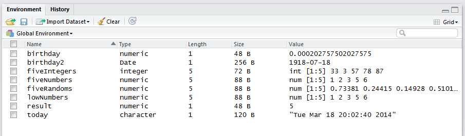
Figure 4.4: The grid view.

The next datatype (storage mode) you should know about is called a “logical” datatype. Let’s create a new vector called fiveBooleans that contains the only the words, TRUE or FALSE, by asking R if the random numbers contained in fiveRandoms are greater than 0.5. We do that by simply entering fiveRandoms > 0.5, which is another example of vectorization: R will evaluate each entry in fiveRandoms, and return the word TRUE if the entry is greater than 0.5 and FALSE if not.

fiveBooleans <- fiveRandoms > 0.5
fiveBooleans

## [1]  TRUE FALSE  TRUE  TRUE  TRUE

Vectorization is an R specialty . . . it allows rapid calculation across each element within an object without the use of loops (a topic covered in later chapters).

Your result will be different than the one listed above because your fiveRandoms object contains different values. If you look at the global environment, you should see that an object called fiveBooleans has been created, and this is a vector of length 5 with a type that is logical. This means it is a vector that contains only TRUE or FALSE entries. Note that TRUE and FALSE are capitalized. In other programming languages, this is known as a “boolean” data type.

We can also create an object of character data type. We’ve already seen that the object we created called today stores character data, but let’s look at another example. R has a built-in object called letters, which stores the letters of the alphabet. Let’s take a look at the letters object, and then assign a new object called letters2 to it:

# look at R's built in object called characters; 
# note that this is not in your Environment
letters

##  [1] "a" "b" "c" "d" "e" "f" "g" "h" "i" "j" "k" "l" "m" "n" "o" "p" "q" "r" "s" "t" "u" "v" "w" "x" "y" "z"

# create a new object called letters2
# set the value to be equal to the value in the object called letters
letters2 <- letters
# get the structure of the object, letters2
str(letters2)

##  chr [1:26] "a" "b" "c" "d" "e" "f" "g" "h" "i" "j" "k" "l" "m" "n" "o" "p" "q" "r" "s" "t" "u" "v" "w" "x" "y" "z"

Look at the letters2 object in the Environment pane; you will see that it is a character type with a length of 26. Also note that each letter is enclosed by quotation marks. Further note R’s display of the letters in the console (yours may look slightly different). Do you see how the first line of output starts with [1]? This means that the returned output begins with the 1st element of the vector. Depending on your screen, your output may spill over into a second line. When multiple lines of output are needed to display the full vector, R tries to help us understand where we are in the vector by providing the “index” associated with the first entry on each line of output.

Can a vector store different types (modes) of data within it? Let’s try it. Create a new object (shoebox) called mixed, that contains 3 elements: “dog”, 10, and TRUE. Here, “dog” is a character, 10 is an integer, and TRUE is a logical datatype. Incidentally, R lets you write “dog” (with a double-quote), as well as ‘dog’ (with a single quote) . . . either is fine as long as you match them . . . both may be necessary if you are nesting quotation marks (e.g. bond <- ‘he said “shaken, not stirred”’ requires different types of quotation marks.

# create an object called mixed, with values "dog", 10, and TRUE
mixed <- c("dog", 10, TRUE)

# look at the object called mixed
mixed

## [1] "dog"  "10"   "TRUE"

You should see that R stores this vector as a character data type. Notice that the number 10 is actually stored as “10”, and the word TRUE is now stored as “TRUE”. The quotation marks around each element is a dead give-away that the object is a character type. Since “10” is now a character, it cannot be used as a number in calculations.

A vector must contain a single data type, and while it is possible to store the number 10 as a character type, it is not possible to store “dog” as a numeric type.

Let’s try another vector with mixed data types:

# create an object called mixed2, with values FALSE, 10, and TRUE
mixed2 <- c(FALSE, 10, TRUE)

# look at the object called mixed2
mixed2

## [1]  0 10  1

In this case, R stores the vector named mixed2 as a numeric type. What happens here is that the logical entries are interpreted as 1’s or 0’s, with TRUE equal to 1 and FALSE equal to 0.

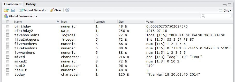
Figure 4.5: The grid view.

The type (mode) of an object tells us how R is storing its content. A related function is called class, which returns the class of an object (which in turn controls how other functions work with the object).

# look at the class function helpfile
help(class)

# find the class for the object called mixed2
class(mixed2)

## [1] "numeric"

The class can also be inferred with the str function: the num output tells us the data are numeric, and the [1:3] output tells us the object is a vector (more on vectors in a minute).

# find the structure of the object called mixed2
str(mixed2)

##  num [1:3] 0 10 1

In our experience, one of the most common mistakes when coding in R occurs when trying to execute a function on objects of a given class when R is expecting something else. The str function is one of your best friends when it comes to R functions; it provides not only the class and a peek at the values as well.

Note: An object can be fully examined by using the class function, the typeof function, and the mode function. Though not always the case, these three functions can return the same result, especially for vectors. We won’t dwell on the differences, but generally speaking typeof and mode provide information about how R is storing an object, while an object’s class determines how it is used in future R calls.

4.3 Changing Data Types

You were just introduced to a number of different data types that can be used in R. One of the neat / nice / convenient things about R is that if you don’t specify a data type, R will guess and assign the type it thinks best one that fits the data (as we saw with mixed value data).

However, there are times when R will guess wrong (particularly when reading data into R), and there are other times when we need a specific data type for the task at hand. For those times, R has coercion functions, which are generally used to convert an existing object to a new type as opposed to creating a new object. Coercion functions start with “as.” and end with the output class. Here are a few that convert objects from one type to another:

as.character - converts to character data types
as.numeric - converts to numeric data types
as.Date - converts to dates
as.factor - converts characters to factors

Let’s practice one of these functions. Let’s practice using one of these functions by creating an object that stores Eleanor Roosevelt’s birthday as a string. Then we’ll change it to both a date data type and a numeric data type:

# create a character string of Eleanor Roosevelt's birthday
eleanor  <- "1884-10-11"
# look at the value of eleanor
str(eleanor)

##  chr "1884-10-11"

# convert to date
eleanor  <- as.Date(eleanor)
# look at the value of eleanor
str(eleanor)

##  Date[1:1], format: "1884-10-11"

# convert to number
eleanor <- as.numeric(eleanor)
# look at the value of eleanor
str(eleanor)

##  num -31127

We bet you weren’t expecting this answer! We’ll cover dates and what -31127 actually means in future chapters (yes, computers store dates as numbers).

R has another data type that we have not mentioned, the factor datatype. Factors look like characters, but they are not stored as characters . . . hence they can be a source of confusion. Factor datatypes are very important if you are planning to do statistical analysis on a dataset, such as a t-test or ANOVA. The easiest way to introduce you to factors in R is to create a vector of characters, change it to factors, and then discuss it.

# create a names vector of the boys in Mrs. Smith's first grade class; 
# note how popular the name "Ben" is in Vermont
boys <- c("Ben", "Alden", "Ben", "Ben", "Max", "Elias", "Evan", "Miles")

# look at the structure; notice that this is a character vector
str(boys)

##  chr [1:8] "Ben" "Alden" "Ben" "Ben" "Max" "Elias" "Evan" "Miles"

# convert the vector to factors
boys  <-  as.factor(boys)

#look at the structure, notice that this is a factor with 5 levels
str(boys)

##  Factor w/ 6 levels "Alden","Ben",..: 2 1 2 2 5 3 4 6

Here an observant user may notice that factors are typically character values, but appear to be stored as an integer code in which each unique integer represents a longer character value. For example, the vector ‘boys’ is of class factor with 6 levels (unique values): “Ben”, “Alden”, “Max”, “Elias”, “Miles”, and “Evan”. From our output, it appears that “Ben” is stored as 2, “Alden” is stored as 1, “Max” is stored as 5, “Elias” is stored as 3, “Evan” is stored as 4, and “Miles” is stored as 6. Thus, each name is mapped to an integer that is stored internally by R. It appears that R has assigned these numbers alphabetically.

The levels functions returns the names of each level.

# look at the levels
levels(boys)

## [1] "Alden" "Ben"   "Elias" "Evan"  "Max"   "Miles"

Note that this returns the common name in the order of their numeric assignment, but does not provide the numeric assignment directly. If you want to see the integer mapping, use the as.integer function:

# convert the factor boys to integers
as.integer(boys)

## [1] 2 1 2 2 5 3 4 6

The take home point is that R is storing the factors as numbers behind the scenes, but there is usually no need to convert factors to integers.

If you want more control over how the mapping from levels to integers is done, use the factor function. In this next example, let’s suppose that you have some integer data from 1:5, and these designate people’s ratings of “Cosmos” on Netflix. Here, we’ll use the sample function to create a dataset called data that consists of 50 viewer ratings. We’ll draw 50 random samples with replacement between 1 and 5, and include the prob argument to establish the probabilities of drawing each number. The use of the ‘prob’ argument can be used to weight how the numbers are drawn….in the code below, there is a 0 probability of drawing a score of 1, a 10% chance of drawing a score of 2….and a 60% chance of drawing a 5. “Cosmos” is a great series!

# create a dataset with 100 values of numbers of 1 to 5 using the sample function; 
data <- sample(x = 1:5, size = 50, replace = T, prob = c(0, 0.1, 0.1, 0.2, 0.6))

# look at the data
data

##  [1] 2 3 5 4 5 5 5 2 4 3 3 4 5 5 2 5 5 5 5 3 4 5 4 5 3 2 5 2 5 4 2 5 3 5 5 5 4 5 5 4 5 3 5 2 2 4 5 5 5 5

# convert the vector to factor and control the levels and labels.
factor(x = data, 
       levels = c(1,2,3,4,5), 
       labels = c("rotten", "poor", "ok", "good", "excellent"))

##  [1] poor      ok        excellent good      excellent excellent excellent poor      good      ok        ok        good      excellent excellent
## [15] poor      excellent excellent excellent excellent ok        good      excellent good      excellent ok        poor      excellent poor     
## [29] excellent good      poor      excellent ok        excellent excellent excellent good      excellent excellent good      excellent ok       
## [43] excellent poor      poor      good      excellent excellent excellent excellent
## Levels: rotten poor ok good excellent

# look at the structure of the data
str(data)

##  int [1:50] 2 3 5 4 5 5 5 2 4 3 ...

You might have noticed that nobody rated “Cosmos” as “rotten”. But nonetheless, the levels argument allows us to specify what “could have been” scored. The labels are important for graphing, as we’ll see in later chapters.

Conversion between some data types is not possible. For example, we noted earlier that we can convert a number to character data, but the converse is not always true. If we try to store character data as numeric data R will not allow it, and will both warn us and then replace all invalid elements with NA values.

# review our object mixed
mixed

## [1] "dog"  "10"   "TRUE"

# attempt to convert it to "numeric"; which elements do you think will be preserved?
mixed.num <- as.numeric(mixed)

## Warning: NAs introduced by coercion

# take a look how we did
mixed.num

## [1] NA 10 NA

So while R will convert “TRUE” to TRUE automatically when evaluating it as a logical, it will not convert “TRUE” to 1 with as.numeric().

As an aside, you might have noticed the name of the object mixed.num includes a period. This is fine, and many coders use a period to separate words in a name. You can also use and underscore if you prefer.

Exercise: Change the Data Types

Coerce the vector c(1,1,0,1,0) to logical TRUE and FALSE values.
Coerce the vector c(1,1,0,1,0) to character values.
Create a vector of 10 values, filled with random numbers between 1 and 100.
Add a random number between 0 and 1 to each value in your vector.
Find your vector’s datatype.
Coerce your vector’s datatype to integers.

This is a great time for a short coffee break.

Figure 4.6: Time to stretch.

4.4 Object Types

We’ve asked you to think of an object like a shoebox – a “thing” that can hold something. But shoeboxes come in different flavors: Nike shoeboxes hold running shoes, while The North Face shoeboxes hold hiking boots, and KEEN shoeboxes hold sandals (more or less). The same goes for objects in R.

There are five main object “classes” that hold different types of data:
1. Vectors
2. Matrices
3. Arrays
4. Lists
5. Dataframes

Actually, there are more than 5, but these are commonly used. The simplest way to give you an overview of these types is to use a spreadsheet analogy.

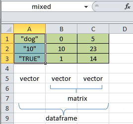
Figure 4.7: R objects in spreadsheet view.

A vector is a single row or column of data. The cells A1:A3 are highlighted, and you can see that this group of cells is named mixed (see the upper left of the figure). This particular vector has three elements within it, and it stores data that have a mode of character. Similarly, cells B1:B3 make up a vector called mixed2. Cells C1:C3 make up another vector (arbitrarily called numbers) that stores numeric datatypes. As we’ve already seen, vectors store only one datatype – they cannot store values with different datatypes.

Cells B1:C3 can be thought of as a matrix object. Matrices can store only a single datatype (usually numbers). Let’s suppose that these cells are called my.matrix. If we could make this matrix have many dimensions (like a cube of numbers), it would be called an array. Arrays can have multiple dimensions, but like matrices, can store only a single datatype. We’ll work with arrays extensively in Chapter 12.

In R, objects can be combined into a list. For example, in the spreadsheet example, we can combine mixed (a vector), mixed2 (a vector), and my.matrix (a matrix) into a new type object, a list. Lists are a very important concept in R. They are collections of objects, sort of like a shoe store – it can hold shoeboxes of all sorts, even other shoe stores! Many functions (like statistical functions) return the results in lists, where each portion of the list holds different kinds of information.

Finally, cells A1:C3 together can be thought of as a dataframe, which is a special type of list that is composed of many different vectors, all of the same length. In this example, our dataframe consists of the three vectors, mixed, mixed2, and numbers.

Each of these object types has unique properties, so we’ll work through them one by one. Keep in mind that we are aiming for the big picture here!

4.5 Vectors

We’ve already made several vectors in R – just look at your work in the Environment tab and look for the square brackets. Do you see the word vector anywhere? We don’t. That’s because a vector is the simplest type of object in R, and we suppose it is the default object type and not worth highlighting this fact in the environment’s grid view. When an object is a vector, the Type column displays the type of data held within the vector (its mode). If you want to verify whether an object is a vector, use the is.vector function, an pass to it the name of the object you wish to test; R will return either TRUE or FALSE depending on whether the object is a vector or not.

We’ve created vectors using the c function, the seq function, the sample function, and the runif function. Let’s create a new vector called my.vector that combines two of our previous vectors. Remember that vectors can store only a single datatype, so we’ll combine two vectors that contain numbers:

# use the c function to combine the two vectors, fiveIntegers and fiveRandoms into a new object called my.vector
my.vector <- c(fiveIntegers,fiveRandoms)

# look at the object 
my.vector

##  [1] 40.0000000 76.0000000 40.0000000 84.0000000 64.0000000  0.6276556  0.4272567  0.9864081  0.6058641  0.5098213

You can see that this is one long vector now stores a numeric datatype. The R output shows all 10 elements, but the display may require multiple lines of output to show them all. If so, keep in mind that the vectors indices can be identified by brackets. For example, the [1] in the first row of the output means the output begins with with the first element of the vector, which is 40.

Now let’s return to our very first example in this primer:

result <- sqrt(10)
result

## [1] 3.162278

It should be clear now that the result, 3.162, is stored in a vector, and R is displaying the first element of this vector.

We can use the length function to find out how many “elements” our vector has:

length(my.vector)

## [1] 10

Now we have a shoebox that is named my.vector, and it has a scrap of paper on it with 10 numbers (in a particular order). How do we open the shoebox to pull a particular number out? We use R’s indexing method for vectors, which are square brackets [ ].

Each of the 10 numbers (or elements) in my.vector has a position within the vector, and R has a specific syntax for pulling certain elements out of the vector object. Here are 6 examples:

To get the first element stored in my.vector, use my.vector[1]
To get the third element stored in my.vector, use my.vector[3]
To get the first three elements stored in my.vector, use my.vector[1:3]
To get elements 3, 5, 7, and 8, use my.vector[c(3,5,7,8)]
To return everything but elements 3, 5, 7, and 8, use my.vector[-c(1,3,7,8)]
To get all of the elements, except the fifth element, use my.vector[-5]
To get the last three elements only, use my.vector[-(1:7)]

Remember that an index is a position within the vector. Since my.vector has 10 elements, the indices are 1 through 10. If we want to select certain indices from my.vector, we can simply identify the ones we want (see examples 1 through 4). Of these, example 4 is “tricky” because my.vector[c(3,5,7,8)] embeds a c function so that we can pull out various combinations of numbers, in the specified order. You’ll find this to be a very, very useful approach. You can’t just type in my.vector[3,5,7,8] because R will think you are trying to extract an element from a four dimensional array!

If we want to exclude certain indices, we use a - symbol, as shown in examples 5 and 6. Example 5 is pretty straightforward: my.vector[-5] means return all elements of my.vector except the fifth element. But example 6 is tricky. The my.vector[-(1:7)] example uses parentheses to surround the numbers 1 through 7. If we didn’t have the parentheses, we would get an error. Try this:

my.vector[-1:7]

Error in my.vector[-1:7] : only 0's may be mixed with negative subscripts

What the error says is an important troubleshooting message! There error says “only 0’s may be mixed with negative subscripts”. A negative subscript indicates exclusion, but -1 is mixed with 7. You can’t omit some indices and select others at the same time. By entering my.vector[-(1:7)], we are telling R to exclude indices 1 through 7.

Quick tip: In the RStudio editor, notice that when you type the opening square bracket [, the Editor automatically adds the closing square bracket. The Editor shows sets of parentheses in the same way. In addition, if the cursor is located immediately after either a parentheses or square bracket, the Editor highlights the corresponding syntax in the text. This is very useful because coding mistakes often occur when a parenthesis or bracket is out of place.

Exercise: Working with Vectors

Create a vector (object) named “family” and enter the names of your (or a fictitious) family. If you have a really small family, you can add some friends in there too. Don’t forget the quotes!
Use the length function to find the length of your vector.
Use the str function to find the structure of this new object.
Use the class function to find the class of the data within the object called “family”.
Extract the shortest family member.
Extract the two oldest family members, and assign them to a new object called “elders”.
Look at the object called “elders”.
Extract the two oldest family members again, but this time reverse their order.
Assign them to a new object called “elders2”.
Look at the object called “elders2”.

We’ve been using the index number (or position within a vector) to refer to data within our vector. But it is also very useful to name the elements within a vector so that you can extract them by name instead of by index. Let’s do that now.

Suppose someone hands you a single shoebox that contains a pair of shoes. Its brand is Nike, the size is 10, and the model is “Pegasus”. We can create an object called shoebox that is a vector, and each element of the vector is named:

# create a new object called shoebox
shoebox <- c(brand = "Nike", size = 10, model = "Pegasus")
# look at the object called shoebox
shoebox

##     brand      size     model 
##    "Nike"      "10" "Pegasus"

By now you should see that the object called shoebox is storing data that are characters. See the quotes? Can you also see that each element is named? The names are also characters (though since they are being displayed as element names, they are not wrapped in quotes). The names are provided in the top row, and we can view them with the names function:

# look at the names of the vector called shoebox
names(shoebox)

## [1] "brand" "size"  "model"

Our shoebox now has some attributes associated with it. From dictionary.com, we see that an attribute is “something attributed as belonging to a person, thing, group, etc.; a quality, character, characteristic, or property.”

Names are just one of many attributes an object can have. We will learn more about attributes later in this chapter.

When elements are named, we can extract by name instead of by index.

# extract the brand
shoebox['brand']

##  brand 
## "Nike"

# this is the same as:
shoebox[1]

##  brand 
## "Nike"

# extract the size and model
shoebox[c('size','model')]

##      size     model 
##      "10" "Pegasus"

# change the size to 11
shoebox['size'] <- 11
# view the object called shoebox
shoebox

##     brand      size     model 
##    "Nike"      "11" "Pegasus"

Exercise: Working with Named Vectors

Think of one of your favorite animals. Create a vector with the name of that animal that contains three elements that describe the animal. Name each element and provide a value.

Use the length function to find the length of your vector.

Use the str function to find the structure of this new object.

Use the class function to find the class of the data within the object you created.

Extract the first element by name.

Extract the first and third elements by name.

Teaser: add one more named element to your vector that describes something new about your animal.

4.6 Matrices

A matrix is a special case of a vector object with two dimensions that stores only one datatype (dimension is another example of an attribute). You can create a matrix easily with the matrix function.

First, let’s look at this function’s helpfile:

help(matrix)

We can focus on the arguments for the matrix function using the args function:

# get the arguments for the function called matrix
args(matrix)

## function (data = NA, nrow = 1, ncol = 1, byrow = FALSE, dimnames = NULL) 
## NULL

This function has several arguments, including data, nrow, ncol. The default values are specified, so if you do not enter an argument, R will use the default values. For example, if you don’t provide the byrow argument, R will use FALSE.

Let’s create a matrix with 3 rows and 2 columns, and fill the matrix with random numbers (uniform random numbers between 0 and 1).

# create a vector 6 random numbers
numbers <- runif(6)

# look at the numbers
numbers

## [1] 0.67683975 0.15292014 0.96226446 0.30098597 0.24984045 0.03126409

# create an object called my.matrix that is a matrix object
my.matrix <- matrix(data = numbers, nrow = 3, ncol = 2)

# look at the object, my.matrix
my.matrix

##           [,1]       [,2]
## [1,] 0.6768397 0.30098597
## [2,] 0.1529201 0.24984045
## [3,] 0.9622645 0.03126409

Because we did not provide the byrow argument, R used the default value, which is FALSE. This means we filled the matrix by column, which you can confirm directly. Since we used the default value of FALSE, R filled in the 6 elements of the matrix on a column-by-column basis. This means we snaked the vector that created the matrix first down column 1 and then down column 2.

What does the [,1] [,2] mean in the first row? That is the header of our matrix. Column 1 is identified as [,1], while column 2 is identified as [,2]. In this bracket notation, the rows are always identified first, followed by a comma, then followed by the column identifier. Remember this order: [Rows, Columns] . . . think of Russell Crowe or Ray Charles. This order might also be familiar if you’ve studied linear algebra. If an identifier is not specified but the comma placeholder is present, it means “all”. So [,1] means “all rows, column 1”, while [,2] means “all rows, column 2”.

The portions [1, ] [2, ] [3,] represent our row headers, where [1, ] means “row 1, all columns” and [2, ] means “row 2, all columns”, and [3, ] means “row 3, all columns”.

Now look for my.matrix in your Global Environment. You should see that the “Type” is listed as matrix. This is its class. You can also tell it is a matrix by looking in the Value column. See the notation [1:3, 1:2]. This notation tells you my.matrix is a 3 row by 2 column matrix, and the num that preceeds it tells you that it stores numeric values (its mode).

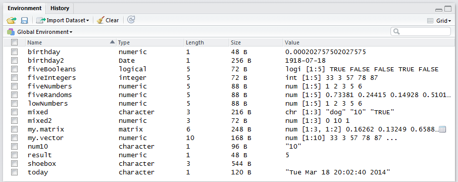
Figure 4.8: The grid view.

Obviously, we just created this matrix, but if we didn’t know much about it, we could use the nrow and ncol functions to get more information about this object.

# get the number of rows for the object called my.matrix
nrow(my.matrix)

## [1] 3

# get the number of columns for the object called my.matrix
ncol(my.matrix)

## [1] 2

The dim function is also useful for returning both answers at once, knowing that the number of rows is always given first, followed by the number of columns. Remember Russell Crowe?

dim(my.matrix)

## [1] 3 2

What if we tried getting the number of columns for one of the vectors we made previously, say, mixed?

ncol(mixed)

## NULL

You can see that R returns NULL. The reason is that we are using a function that is meant for objects that have multiple dimensions, and not one-dimensional vectors.

What about length?

length(my.matrix)

## [1] 6

Here’s another surprise, but this one is important. At its core, a matrix is a vector (with dimension attributes). The function length pertains to vectors, and since matrices are vectors with dimensional attributes, length returns the count of elements in the matrix. Think of a matrix as a vector that “snakes” around the rows and columns in a specified direction. For example, you can ask R to return all of the elements in the matrix using vector notation as follows:

my.matrix[1:6]

## [1] 0.67683975 0.15292014 0.96226446 0.30098597 0.24984045 0.03126409

Looks like a vector, right?

You can never go wrong by using the trusty str function; it will provide the dimensions. Just don’t get thrown off when you see that the values in your matrix are different from ours. Recall that they were generated randomly with the runif function!

str(my.matrix)

##  num [1:3, 1:2] 0.677 0.153 0.962 0.301 0.25 ...

Here, the output [1:3, 1:2] suggests that the object type is a matrix. The first section 1:3 is for Rows, and the section 1:2 gives us the Column, separated by a comma. This suggests that to extract data out of this object, we will need to specify the row index and the column index, separated by a comma. We’ll refer to this matrix indexing throughout this primer. Let’s try it:

# extract from the object, my.matrix,  the element stored in row 2, column 2 
my.matrix[2, 2]

## [1] 0.2498404

# extract from the object, my.matrix, the element stored in row 1, column 1
my.matrix[1, 1]

## [1] 0.6768397

# extract row 2, all columns from the object, my.matrix
my.matrix[2, ]

## [1] 0.1529201 0.2498404

# extract all rows, but only column 1 from the object, my.matrix
my.matrix[, 1]

## [1] 0.6768397 0.1529201 0.9622645

When you want to include all of the rows, or all of the columns from a matrix, as we did in the last two examples, just leave the index number off.

If we want to get all values in the first column but forget to add the comma placeholder, we end up with [1], which is vector indexing for the first element of the matrix.

my.matrix[1]

## [1] 0.6768397

Unless that is what you want, don’t forget the comma!

If the last two examples seem to be too vague (a blank space before or after a column), you could add in the built in names for rows and columns, like this:

# extract row 2, all columns from the object, my.matrix
my.matrix[row = 2, column =]

## [1] 0.1529201 0.2498404

# extract all rows, but only column 1 from the object, my.matrix
my.matrix[row = , column = 1]

## [1] 0.6768397 0.1529201 0.9622645

Did you notice the argument called dimnames when you created your matrix? We omitted that argument too, but now let’s add it.

Go back to the matrix function helpfile, and review the example for creating a matrix. We’ll alter this helpfile example a tiny bit by adding in some additional argument names.

# from the matrix function helpfile:  create a new object that is a matrix with the name mdat
mdat <- matrix(c(1,2,3, 11,12,13), 
               nrow = 2, 
               ncol = 3, 
               byrow = TRUE,
               dimnames = list(c("row1", "row2"), c("C.1", "C.2", "C.3")))

# same code but with rows and columns argument names included
mdat <- matrix(data=c(1,2,3, 11,12,13), 
               nrow = 2, 
               ncol = 3, 
               byrow = TRUE,
               dimnames = list(rows = c("row1", "row2"), columns = c("C.1", "C.2", "C.3")))

Let’s work through this code, and use a visual aid to guide us:

Figure 4.9: Creating a matrix in R.

We use the matrix function to create a matrix with 2 rows and 3 columns. We will fill the 6 elements of the matrix with the numbers 1, 2, 3, 11, 12, 13. These will be filled by rows (so 1, 2, and 3 will occupy row 1; 11, 12, and 13 will occupy row 2). The dimnames argument will be used to name the rows and columns, and we’ll store the names in a list (the shoestore), which is what is required by the dimnames argument. Russell Crowe is telling us that we need to name the rows first, and we’ll use the c function to create a vector called “rows”, and pass in the elements “row1” and “row2”. We’ll use a second c function to create another vector called “columns” to name the columns “C.1”, “C.2”, and “C.3”. Notice that the names are stored in a list (a type of object), and that the actual row and column names must be character datatypes (in quotes). Let’s have a look at our newly created matrix:

# look at mdat
mdat

##       columns
## rows   C.1 C.2 C.3
##   row1   1   2   3
##   row2  11  12  13

Take a look at mdat in your environment, and carefully examine its type, length, size and value.

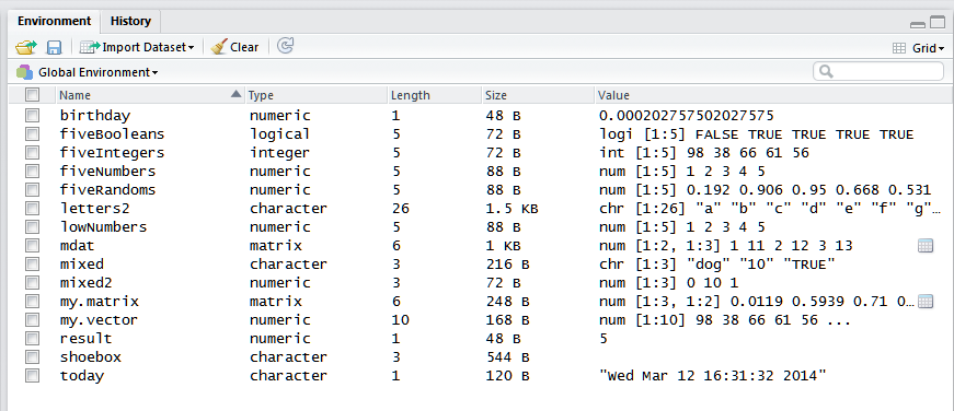
Figure 4.10: Creating a matrix in R.

Now we can use the names of the rows and columns to extract data from our object. Don’t forget that a comma must be supplied to separate the rows and columns, and don’t forget that names are characters that must be supplied with quotes!

# extract row 1 from the matrix named mdat, all columns
mdat["row1",]

## C.1 C.2 C.3 
##   1   2   3

# extract row 1, column 2 from the matrix named mdat
mdat["row1", "C.2"]

## [1] 2

Now let’s look at this object’s structure.

str(mdat)

##  num [1:2, 1:3] 1 11 2 12 3 13
##  - attr(*, "dimnames")=List of 2
##   ..$ rows   : chr [1:2] "row1" "row2"
##   ..$ columns: chr [1:3] "C.1" "C.2" "C.3"

The output here is here is very revealing (good old str!). We see the word num which indicates that the data are numeric. We see [1:2, 1:3] which gives us the dimensions of the matrix. We then see the 6 elements that constitute the matrix.

We also see attr(*,“dimnames”)=List of 2. What on earth is this? When we created our matrix, we created an attribute for our object called dimnames. This attribute, in turn, is a list that contains two vectors (List of 2). Remember that a list is the shoestore…a list can hold vectors, arrays, matrices, and even other lists! This list holds two vectors. The first vector is called rows, which is a vector of characters with elements “row1” and “row2”. The second vector is called columns, which is a vector of characters with elements “C.1”, “C.2”, and “C.3”. Each part of the list begins with a dollar sign $.

We will talk about attributes and lists in a few minutes. (If you’re inclined, try re-running the code, but set the by.row argument to FALSE and see what happens!).

Exercise:

Create a 3*2 matrix with random integers between 30 and 50.
Name the rows Winken, Blinken, and Nod. Name the columns Height and Weight.
Extract the height of Winken.
Extract the weight of Nod.
Find the average weight with the mean function.

4.7 Arrays

Array objects are very similar to matrices, except that they can have more than two dimensions. You can build an array with the array function.

# look at the array function's helpfile
help(array)

# look at the arguments of the array function
args(array)

## function (data = NA, dim = length(data), dimnames = NULL) 
## NULL

Notice that the argument names are very similar to the matrix function: data is the data you want to fill into the cells or elements, dim gives the dimensions, and dimnames lets you name the dimensions.

Let’s create an array called tauntauns, that tracks the number of individuals through 5 years, ages 0 through 10, and both sexes (male and female). We’ll fill this array with 0’s to begin with, and then will populate the array with random numbers. We’ll need 5 * 11 * 2 = 110 random numbers to fill the entire array. There are 11 age classes because we include 0 year olds.

# create an object called tauntauns that is an array
tauntauns  <- array(data = 0, 
                     dim = c(5,11,2), 
                     dimnames = list(year = 1:5, age = 0:10 , sex = c("male", "female")))
# look at the object called tauntauns
tauntauns

## , , sex = male
## 
##     age
## year 0 1 2 3 4 5 6 7 8 9 10
##    1 0 0 0 0 0 0 0 0 0 0  0
##    2 0 0 0 0 0 0 0 0 0 0  0
##    3 0 0 0 0 0 0 0 0 0 0  0
##    4 0 0 0 0 0 0 0 0 0 0  0
##    5 0 0 0 0 0 0 0 0 0 0  0
## 
## , , sex = female
## 
##     age
## year 0 1 2 3 4 5 6 7 8 9 10
##    1 0 0 0 0 0 0 0 0 0 0  0
##    2 0 0 0 0 0 0 0 0 0 0  0
##    3 0 0 0 0 0 0 0 0 0 0  0
##    4 0 0 0 0 0 0 0 0 0 0  0
##    5 0 0 0 0 0 0 0 0 0 0  0

When we look at this object, we can see that the years are given in the rows, which we specified as our first dimension, dim = c(5,11,2). The ages are given by the columns, which we specified as our second dimension, dim = c(5,11,2). Because we have a third dimension, this array is shown in two blocks, one for males and one for females. In total, there are 110 cells of data.

Look for the object called tauntauns in your Environment. Can you see that it’s type is listed as “array”?

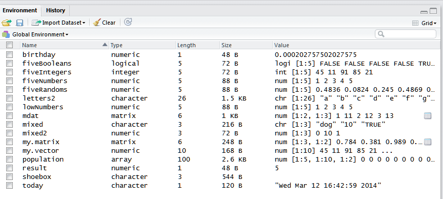
Figure 4.11: The grid view.

Now let’s generate 110 random numbers between 100 and 500 with the help of the sample function. This will result in a new object called individuals, which is a vector containing numbers that represent the number of individuals of a given age and sex in a given year. Then, we’ll replace the 0’s in the tauntauns array with the numbers stored in individuals. The notation here is tauntauns[,,]. Can you see why? Just like the matrix had dimensions that were separated by commas, so too the array has dimensions separated by commas. Here, with no entries between the commas, it means “select all of the years, select all of the ages, and select both of the sexes, then fill them in with a random number between 100 and 500.” Make sure to look for the “snaking” route in this example.

# replace the 0's with random numbers between 100 and 500
individuals  <-  sample(x = c(100:500), size = 110)

# look at the individuals
individuals

##   [1] 193 401 350 346 439 267 344 275 166 431 175 224 192 150 488 484 161 204 214 418 262 318 403 317 465 121 291 293 239 311 306 209 479 362 461 463
##  [37] 377 498 115 307 440 236 428 444 219 230 100 446 392 131 353 330 313 237 257 108 412 449 478 273 220 149 325 339 112 468 264 432 176 173 248 256
##  [73] 464 476 146 378 272 269 399 102 229 452 410 487 460 206 154 500 165 181 489 163 184 402 462 194 250 331 340 309 172 387 235 289 442 314 327 244
## [109] 373 315

# replace the array 0's with random numbers
tauntauns[,,]  <- individuals

# look at the object called tauntauns
tauntauns

## , , sex = male
## 
##     age
## year   0   1   2   3   4   5   6   7   8   9  10
##    1 193 267 175 484 262 121 306 463 440 230 353
##    2 401 344 224 161 318 291 209 377 236 100 330
##    3 350 275 192 204 403 293 479 498 428 446 313
##    4 346 166 150 214 317 239 362 115 444 392 237
##    5 439 431 488 418 465 311 461 307 219 131 257
## 
## , , sex = female
## 
##     age
## year   0   1   2   3   4   5   6   7   8   9  10
##    1 108 220 468 248 378 229 206 489 194 172 314
##    2 412 149 264 256 272 452 154 163 250 387 327
##    3 449 325 432 464 269 410 500 184 331 235 244
##    4 478 339 176 476 399 487 165 402 340 289 373
##    5 273 112 173 146 102 460 181 462 309 442 315

Let’s use the str function to look at the information associated with this object:

# look at the structure of tauntauns
str(tauntauns)

##  num [1:5, 1:11, 1:2] 193 401 350 346 439 267 344 275 166 431 ...
##  - attr(*, "dimnames")=List of 3
##   ..$ year: chr [1:5] "1" "2" "3" "4" ...
##   ..$ age : chr [1:11] "0" "1" "2" "3" ...
##   ..$ sex : chr [1:2] "male" "female"

The first section of this output, num [1:5, 1:11, 1:2] gives us the dimensions of our array, and tells us that the array is storing numbers. Once again, we see that our object called tauntauns has an attribute called “dimnames”. This attribute is a list with three sections (List of 3), and the sections are identified as year, age, and sex. Notice the dollar signs that identify each part, and that the names are all in quotes.

To extract information from the array, we need to specify all three dimensions. We can do this in a few different ways:

# extract the female data for all years and all ages
tauntauns[year = ,age = , sex = 'female']

##     age
## year   0   1   2   3   4   5   6   7   8   9  10
##    1 108 220 468 248 378 229 206 489 194 172 314
##    2 412 149 264 256 272 452 154 163 250 387 327
##    3 449 325 432 464 269 410 500 184 331 235 244
##    4 478 339 176 476 399 487 165 402 340 289 373
##    5 273 112 173 146 102 460 181 462 309 442 315

# extract the female data for all years and all ages, but omit the names of the indices
tauntauns[, , 'female']

##     age
## year   0   1   2   3   4   5   6   7   8   9  10
##    1 108 220 468 248 378 229 206 489 194 172 314
##    2 412 149 264 256 272 452 154 163 250 387 327
##    3 449 325 432 464 269 410 500 184 331 235 244
##    4 478 339 176 476 399 487 165 402 340 289 373
##    5 273 112 173 146 102 460 181 462 309 442 315

# extract year 3 
tauntauns[year = 3, ,]

##     sex
## age  male female
##   0   350    449
##   1   275    325
##   2   192    432
##   3   204    464
##   4   403    269
##   5   293    410
##   6   479    500
##   7   498    184
##   8   428    331
##   9   446    235
##   10  313    244

# extract the number of 2 year olds; 
# notice that quotes are needed because "2" is a name
tauntauns[year = , age = "2", sex = ]

##     sex
## year male female
##    1  175    468
##    2  224    264
##    3  192    432
##    4  150    176
##    5  488    173

# extract the 2nd index for age; watch the indexing here: 
# 2 is the second index (which is "1" year olds), whereas "2" year olds are index 3
tauntauns[, 2, ]

##     sex
## year male female
##    1  267    220
##    2  344    149
##    3  275    325
##    4  166    339
##    5  431    112

# extract the number of 1 and 3 year old males in year 3
tauntauns[year = 3,age = c("1","3"), sex = 'male']

##   1   3 
## 275 204

# extract the year 3 data by position
tauntauns[3, , ]

##     sex
## age  male female
##   0   350    449
##   1   275    325
##   2   192    432
##   3   204    464
##   4   403    269
##   5   293    410
##   6   479    500
##   7   498    184
##   8   428    331
##   9   446    235
##   10  313    244

# extract the year 3 data by name
tauntauns[year = "3" , ,]

##     sex
## age  male female
##   0   350    449
##   1   275    325
##   2   192    432
##   3   204    464
##   4   403    269
##   5   293    410
##   6   479    500
##   7   498    184
##   8   428    331
##   9   446    235
##   10  313    244

# extract the number of 2 year olds (which are the third age group)
tauntauns[, 3, ]

##     sex
## year male female
##    1  175    468
##    2  224    264
##    3  192    432
##    4  150    176
##    5  488    173

Double check your work to make sure you’re getting the result you should! You must know (and understand) the order of the array’s dimensions. And you must always be careful to use quotes when selecting data based upon a dimensional attribute as opposed to selecting data based on the index. Again, the str function can come to the rescue.

Exercise: Extracting from an Array

Extract the following pieces of information from the object, tauntauns:

Extract age 10
Extract males of age 10
Extract males of age 10 in year 4
Extract females of ages 1:3
Change the number of males, age 2, year 5 to 100
Find the total population size in year 5
Find the total male population size in year 2
Extract age 4 males in year 3 by index.
Extract age 4 males in year 3 by name.

R has another type of object called a table, which is an array of integer values. Objects of class table can be created from, of all things, the table function, which builds contingency tables for factor datatypes. We’ll use see tables in use in future chapters.

4.8 Lists

We’ve briefly touched on lists, and you’ve already created some lists when you named your matrix and array dimensions. Now let’s look at lists in more detail. If objects are shoeboxes, lists are shoe stores. A list is, well, a list or collection of different objects. The objects can be vectors, matrices, arrays, or even other lists. The main thing to know about lists is that they are “layered” or hierarchical, so to add new objects to a list, or to extract objects from a list, you need to specify even more information than when you extract information from an matrix or array.

Let’s create a list (using the list function) called my.list that is a combination of the objects fiveIntegers, today, and mdat:

# create a list object called my.list
my.list  <- list(fiveIntegers, mdat, today)

Look for the new object, my.list, in your Environment, and you’ll see that this list holds three objects.

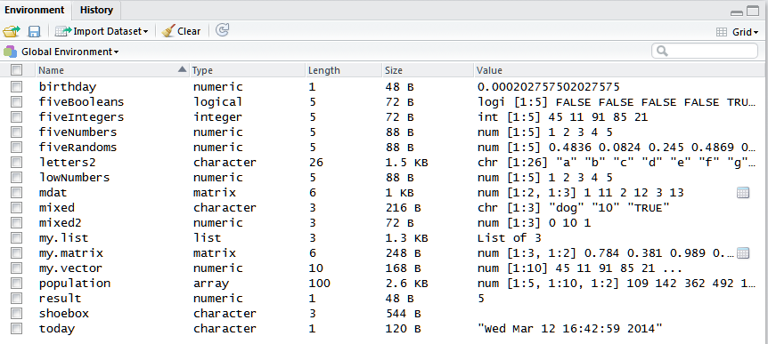
Figure 4.12: my.list is a list of 3 objects.

Do you see a magnifying glass to the right of the Value column? Click on that

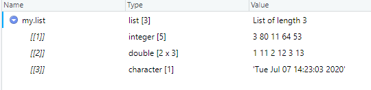
Figure 4.13: Use the magnifier to inspect the list.

Now let’s take a look at your object, my.list, with code:

# look at the object called my.list
my.list

## [[1]]
## [1] 40 76 40 84 64
## 
## [[2]]
##       columns
## rows   C.1 C.2 C.3
##   row1   1   2   3
##   row2  11  12  13
## 
## [[3]]
## [1] "Wed Jan 06 09:01:05 2021"

This looks a bit ugly, but look for the double brackets [[ ]] . When you see double brackets, you know you are working with a list. You already know that our list has three parts to it. Can you see [[1]], [[2]], and [[3]]? These identify the objects that make up the list: [[1]] is the vector fiveIntegers, [[2]] is the matrix mdat, and [[3]] is the vector today. We didn’t name the sections of this list, so the indices are numbered.

To extract information from a list, first you must point to the index in the highest level of the list with the double brackets:

# extract the first part of my.list
my.list[[1]]

## [1] 40 76 40 84 64

# extract the third part of my.list
my.list[[3]]

## [1] "Wed Jan 06 09:01:05 2021"

Note that the double bracket notation will extract the list element, and return its original class:

class(my.list[[3]])

## [1] "character"

Alternatively, if you want to return a list, use the single bracket extractor on a list object:

new <- my.list[3]
class(new)

## [1] "list"

List indexing can be confusing, but it can be conquered with practice. If you want to extract the first integer in fiveIntegers, you would need to first point to extract the section of the my.list that contains the object fiveIntegers (a vector), and then do the subsetting of fiveIntegers, like this:

my.list[[1]][1]

## [1] 40

Note that if you were to extract a subset of data from the second object in the list (which is a matrix), you would need to use matrix notation (good old Russell Crowe again). For example:

my.list[[2]][,"C.1"]

## row1 row2 
##    1   11

If you named the elements of your list, you can extract its pieces with the $ notation, which is equivalent to [[]].

# create a list object called my.list
my.list  <- list("integers" = fiveIntegers, "matrix" = mdat, "today" = today)

# look at the structure of my.list
str(my.list)

## List of 3
##  $ integers: int [1:5] 40 76 40 84 64
##  $ matrix  : num [1:2, 1:3] 1 11 2 12 3 13
##   ..- attr(*, "dimnames")=List of 2
##   .. ..$ rows   : chr [1:2] "row1" "row2"
##   .. ..$ columns: chr [1:3] "C.1" "C.2" "C.3"
##  $ today   : chr "Wed Jan 06 09:01:05 2021"

Here, you see the list but the objects are identified like this: $ integers:, $ matrix:, and $ today:. The dollar sign precedes the name of each section, and you can use this method to extract portions of your list, like this:

# extract the portion of my.list that is named integers
my.list$integers

## [1] 40 76 40 84 64

You can also use this method:

# we can extract the section named "integers" by referencing in the two square brackets
my.list[['integers']]

## [1] 40 76 40 84 64

The dollar sign separates the name of the list (my.list) and the element in the list that you want (integers). We will get a lot of practice using lists in future chapters.

Exercise:

Create a list of 4 objects that are in your global environment.
Name the sections of your list.
Extract the first element of the list (the entire object).
Extract from this list the first element WITHIN the first object in your list.

4.9 Data frames

The last object type that we’ll mention is a data frame, which is a list of vectors that all have the same length. Most datasets are stored as data frames in R, and we’ll get a lot of practice using them in the following chapters. For now, though, let’s combine the three vectors, fiveIntegers, fiveBooleans, and fiveRandoms into a data frame with the data.frame function. Let’s take a look at the help file:

# look at the data.frame function helpfile
help(data.frame)

Data frames are lists of vectors, but the vectors themselves can be different data types. (We already know that, within a vector, there can be only one data type, or mode).

# create a dataframe called my.data
my.data <- data.frame(fiveIntegers, fiveBooleans, fiveRandoms)

#  look at the data
my.data

##   fiveIntegers fiveBooleans fiveRandoms
## 1           40         TRUE   0.6276556
## 2           76        FALSE   0.4272567
## 3           40         TRUE   0.9864081
## 4           84         TRUE   0.6058641
## 5           64         TRUE   0.5098213

Now let’s use the rownames and colnames functions, which do what their name implies:

# look at the column names of the dataframe, my.data
colnames(my.data)

## [1] "fiveIntegers" "fiveBooleans" "fiveRandoms"

# look at the row names of the dataframe, my.data
rownames(my.data)

## [1] "1" "2" "3" "4" "5"

Data frames have row names and column names that are characters. You can see that data frames are two dimensional, so to extract information from them, you must specify both the rows and columns. Let’s use the trusty str function to get more information about this new object:

# look at the structure of my.data
str(my.data)

## 'data.frame':	5 obs. of  3 variables:
##  $ fiveIntegers: int  40 76 40 84 64
##  $ fiveBooleans: logi  TRUE FALSE TRUE TRUE TRUE
##  $ fiveRandoms : num  0.628 0.427 0.986 0.606 0.51

The output is telling us that this data frame has 5 observations (rows) with 3 variables (columns). It then walks us through each column, in order, providing the data type of each column and the first few records within the column.

We won’t say more about data frames here because you’ll soon be working with them extensively.

4.10 Changing an Object’s Class

By now you know that R has a number of object classes, and you have practiced creating objects of various sorts. There may be times when we need a specific object type for the task at hand. For those times, R has coercion functions, which are generally used to convert an existing object to a new type as opposed to creating an entirely new object from scratch. We’ve seen a number of coercion functions that change datatypes (modes); recall that the coercion functions start with “as.” and end with the output class. Here are a few that convert objects from one type to another:

as.data.frame - converts an object to a data frame
as.list - converts an object to a list
as.matrix - converts an object to a matrix
as.vector - converts an object to a vector
as.array - converts an object to an array

To see the coercion functions available to you, type as. into your console and press tab key once. Depending on what packages you have loaded, you may see 125 or more coercion functions! Most of them are not meant to be called by the user (you!), but are called by a core function behind the scenes.

Let’s revisit some of the objects we made earlier. Let’s convert my.matrix to a dataframe:

# look at the object, my.matrix
my.matrix

##           [,1]       [,2]
## [1,] 0.6768397 0.30098597
## [2,] 0.1529201 0.24984045
## [3,] 0.9622645 0.03126409

# look at the structure of my.matrix
str(my.matrix)

##  num [1:3, 1:2] 0.677 0.153 0.962 0.301 0.25 ...

# convert my.matrix to a dataframe 
my.matrix  <- as.data.frame(my.matrix)

# look at the structure of my.matrix
str(my.matrix)

## 'data.frame':	3 obs. of  2 variables:
##  $ V1: num  0.677 0.153 0.962
##  $ V2: num  0.301 0.2498 0.0313

This worked out fine (assuming that a dataframe is what you want!). Also note how R named the rows and columns for you:

my.matrix

##          V1         V2
## 1 0.6768397 0.30098597
## 2 0.1529201 0.24984045
## 3 0.9622645 0.03126409

When row and column names are not provided by you, R will name each row of a new with dataframe numerical characters (i.e. 1, 2, 3, etc.), and name each column as V1, V2, V3, etc… (in reference to the fact that in dataframes, columns are typically the Variables of our data).

There are cases, however, where certain objects cannot be coerced to another. Let’s change our vector fiveIntegers to a dataframe, and then try to turn it back into a vector:

# turn the vector fiveIntegers into a dataframe
fiveIntegers  <- as.data.frame(fiveIntegers)
# look at the structure of fiveIntegers
str(fiveIntegers)

## 'data.frame':	5 obs. of  1 variable:
##  $ fiveIntegers: int  40 76 40 84 64

# now try to change it back to a vector
fiveIntegers  <- as.vector(fiveIntegers)

# still a dataframe!
str(fiveIntegers)

## 'data.frame':	5 obs. of  1 variable:
##  $ fiveIntegers: int  40 76 40 84 64

# convert the dataframe to a matrix
fiveIntegers  <- as.matrix(fiveIntegers)

# look at the structure, note that it is a matrix
str(fiveIntegers)

##  int [1:5, 1] 40 76 40 84 64
##  - attr(*, "dimnames")=List of 2
##   ..$ : NULL
##   ..$ : chr "fiveIntegers"

# now convert from matrix to vector
fiveIntegers  <- as.vector(fiveIntegers)

# look at the structure, note that it is a vector
str(fiveIntegers)

##  int [1:5] 40 76 40 84 64

Exercise: Change the Object Types

Create a 3 by 3 matrix filled with random numbers between 1 and 100
Coerce your matrix to a data frame
Coerce your new data frame back to a matrix
Create a new vector consisting of 10 elements
Create a new list that contains your matrix and your vector
Coerce the tauntauns: sex=“female” array to a matrix

4.11 S3 versus S4 Objects

We’ve been talking about objects as shoeboxes (e.g., you created an object called fiveNumbers which contains five integers. By now you know that different objects store different types of information. This metaphor works, generally, but we can take it one step further. All of the objects we have discussed so far are called S3 objects. Think of these objects as cardboard shoeboxes in that they are flexible with respect to the functions that operate on them. For instance, the function called print is actually a generic function that first finds out what class of object is to be printed, then calls the appropriate function for printing. For example, print.factor will print objects that are factors, while print.table will print objects that are tables. With S3 objects, you can use the generic function and R will dispatch the appropriate function.

Another class of objects are called S4 objects. Think of these as steel shoeboxes. They are inflexible and require specific functions to work on them. We won’t delve into S3 vs S4 objects too much here, but we will create some S4 objects in chapter 6 and explore their properties with the str function.

4.12 Attributes

Before we end this chapter, it’s worth delving into the concept of attributes a bit more. Objects, whether they are arrays, matrices, data frames, vectors, or lists, have attributes. These attributes appear when you use the str function. We’ve already created an attribute for some objects called dimnames. But you can also add as many attributes to an object as you’d like. Here’s an excerpt from the R website:

“All objects except NULL can have one or more attributes attached to them. Attributes are stored as a pairlist where all elements are named, but should be thought of as a set of name=value pairs. A listing of the attributes can be obtained using attributes and set by attributes<-, individual components are accessed using attr and attr<-.”

Besides str, you can use the attributes function to list all of an object’s attributes. Let’s take a look at the array object we created called ‘tauntauns’:

# look at the attributes of the object called tauntauns
attributes(tauntauns)

## $dim
## [1]  5 11  2
## 
## $dimnames
## $dimnames$year
## [1] "1" "2" "3" "4" "5"
## 
## $dimnames$age
##  [1] "0"  "1"  "2"  "3"  "4"  "5"  "6"  "7"  "8"  "9"  "10"
## 
## $dimnames$sex
## [1] "male"   "female"

# and of course the structure function works well too!
str(tauntauns)

##  num [1:5, 1:11, 1:2] 193 401 350 346 439 267 344 275 166 431 ...
##  - attr(*, "dimnames")=List of 3
##   ..$ year: chr [1:5] "1" "2" "3" "4" ...
##   ..$ age : chr [1:11] "0" "1" "2" "3" ...
##   ..$ sex : chr [1:2] "male" "female"

A second function you should know about is the attr function. It can be used to retrieve specific attributes of an object:

attr(x = tauntauns, which = "dimnames")

## $year
## [1] "1" "2" "3" "4" "5"
## 
## $age
##  [1] "0"  "1"  "2"  "3"  "4"  "5"  "6"  "7"  "8"  "9"  "10"
## 
## $sex
## [1] "male"   "female"

This same function can be used to create new attributes:

attr(x = tauntauns, which = "comment" )  <- "This is my tauntaun population array"
attr(x = tauntauns, which = "created.by")  <- "Created by me"

This comes in handy for large objects that you create that require metadata, or information about the object, that is connected to the object itself. Note that for many types of objects, attributes will not be shown when you call the object. Rather, you need to use the attributes function to view them. However, for arrays, attributes will be displayed just by calling the object.

4.13 Summary and A Little Pep Talk

That was a whirlwind tour of objects in R. We’ve talked about various datatypes, including numeric, integer, character, logical, factor, and date modes. We’ve also reviewed five main object “classes” that hold different kinds of data:

Vectors - one dimensional series of elements that are all of the same mode.
Matrices - two dimensional series of elements that are all of the same mode.
Arrays - multi-dimensional series of elements that are all of the same mode.
Lists - groups or bundles of different objects.
Dataframes - a special kind of list which is composed of a series of vectors, each of the same length.

There are a few other kinds of objects as well, but these are the main classes that we’ll work with in this primer. It can be overwhelming to remember the different datatypes, the different object types, and the different functions that can be used for each. But you’ll make rapid progress if you keep these points in mind:

When you create an object, always look in your Environment and see what is there.
If you need to remember ONLY one function when it comes to objects, keep str in your back pocket. It returns the datatype, the object type, and lists all of the object’s attributes.
For functions, the help function can never be overused.
Objects have attributes, and the attr and attributes functions can be extremely helpful.

It may also be useful to peak at some of the following cheatsheets, and post those of interest by your computer:

In the next set of chapters, we’ll put on our Tauntaun biologist hats, and begin using R for data analysis and report writing. Onward!

4.14 Answers to Exercise

Always remember that in R, there are several ways to skin a cat. You may have arrived at different solutions to the exercises, and that’s fine! Below, we give examples of how the exercises could have been coded.

Exercise: Change the Datatypes

Coerce the vector c(1,1,0,1,0) to logical TRUE and FALSE values.
Coerce the vector c(1,1,0,1,0) to character values.
Create a vector of 10 values, filled with random numbers between 1 and 100.
Add a random number between 0 and 1 to each value in your vector.
Find your vector’s datatype.
Coerce your vector’s datatype to integers.

# this creates a numeric vector
my.vector  <- c(1,1,0,1,0)

str(my.vector)

##  num [1:5] 1 1 0 1 0

# coerce to logical
my.vector2  <- as.logical(my.vector)

# Coerce the vector c(1,1,0,1,0) to character values
my.vector3  <- as.character(my.vector)

# Create a vector of 10 values, filled with random numbers between 1 and 100. 
my.vector4  <- sample(x = 1:100, size = 10,replace = T)

#Add a random number between 0 and 1 to each value in your vector.  
randoms  <- runif(n = 100)

my.vector5  <- my.vector4 + randoms

# Find you vector's datatype. 
class(my.vector5)

## [1] "numeric"

# Coerce your vector's datatype to integers. 
my.vector6 <- as.integer(my.vector5)

Exercise: Working with Vectors

Create a vector (object) named “family” and enter the names of your (or a fictitious) family. If you have a really small family, you can add some friends in there too. Don’t forget the quotes!
Use the length function to find the length of your vector.
Use the str function to find the structure of this new object.
Use the class function to find the class of the data within the object called “family”.
Extract the shortest family member.
Extract the two oldest family members, and assign them to a new object called “elders”.
Look at the object called “elders”.
Extract the two oldest family members again, but this time reverse their order.
Assign them to a new object called “elders2”.
Look at the object called “elders2”.

# Create a vector (object) named "family" and enter the names of your (or a fictitious) family
family  <- c("Gilligan", "Skipper", "MaryAnn", "Professor", "Ginger", "Lovey", "Thurston")

# Use the `length` function to find the length of your vector
length(family)

## [1] 7

# Use the `str` function to find the structure of this new object
str(family)

##  chr [1:7] "Gilligan" "Skipper" "MaryAnn" "Professor" "Ginger" "Lovey" "Thurston"

# Use the `class` function to find the class of the data within the object called "family".
class(family)

## [1] "character"

# Extract the shortest family member.
family[1]

## [1] "Gilligan"

# Extract the two oldest family members, and assign them to a new object called "elders".
elders  <- family[6:7]
elders

## [1] "Lovey"    "Thurston"

# Extract the two oldest family members again, but this time reverse their order. 
elders2  <- family[7:6]

# Look at the object called "elders2".
elders2

## [1] "Thurston" "Lovey"

Exercise: Working with Named Vectors

Think of one of your favorite animals. Create a vector with the name of that animal that contains three elements that describe the animal. Name each element and provide a value.
Use the length function to find the length of your vector.
Use the str function to find the structure of this new object.
Use the class function to find the class of the data within the object you created.
Extract the first element by name.
Extract the first and third elements by name.
Teaser: add one more named element to your vector that describes something new about your animal.

# Think of one of your favorite animals. Create a vector with the name of that animal that contains 
# three elements that describe the animal.  Name each element and provide a value. 
leatherback.turtle  <- c(diet="jellyfish", clutches = 7, clutch.size = 80)

# Use the `length` function to find the length of your vector
length(leatherback.turtle)

## [1] 3

# Use the `str` function to find the structure of this new object; note our example forces all 
# elements to be characters
str(leatherback.turtle)

##  Named chr [1:3] "jellyfish" "7" "80"
##  - attr(*, "names")= chr [1:3] "diet" "clutches" "clutch.size"

# Use the `class` function to find the class of the data within the object you created.
class(leatherback.turtle)

## [1] "character"

# Extract the first element by name.
leatherback.turtle["diet"]

##        diet 
## "jellyfish"

# Extract the first and third elements by name.
leatherback.turtle[c("diet", "clutch.size")]

##        diet clutch.size 
## "jellyfish"        "80"

# Teaser:  add one more named element to your vector that describes something new about your animal.
leatherback.turtle["status"]  <- "endangered"
leatherback.turtle

##         diet     clutches  clutch.size       status 
##  "jellyfish"          "7"         "80" "endangered"

Exercise:

Create an 3 by 2 matrix with random integers between 30 and 50.
Name the rows Winken, Blinken, and Nod. Name the columns Height and Weight.
Extract the height of Winken.
Extract the weight of Nod.
Find the average weight with the mean function.

# Create an 3 by 2 matrix with random integers between 30 and 50.
numbers  <- sample(x = 30:50, size = 3 * 2, replace = T)
new.matrix  <- matrix(data = numbers,nrow = 3, ncol = 2, byrow = T)

# Name the rows Winken, Blinken, and Nod. Name the columns Height and Weight.
dimnames(new.matrix) <- list(rows=c("Winken", "Blinken", "Nod"), cols = c("Height", "Weight"))
new.matrix

##          cols
## rows      Height Weight
##   Winken      44     37
##   Blinken     42     47
##   Nod         50     39

# Extract the height of Winken
(winken.ht  <- new.matrix['Winken','Height'])

## [1] 44

# Extract the weight of Nod.
(nod.wt  <- new.matrix['Nod','Weight'])

## [1] 39

# Find the average weight with the mean function.
(ave.weight  <- mean(new.matrix[,"Weight"]))

## [1] 41

Exercise: Extracting from an Array

Extract the following pieces of information from the object, tauntauns:

Extract age 10
Extract males of age 10
Extract males of age 10 in year 4
Extract females of ages 1:3
Change the number of males, age 2, year 5 to 100
Find the total population size in year 5
Find the total male population size in year 2
Extract age 4 males in year 3 by index.
Extract age 4 males in year 3 by name.

# remind ourselves about the array tauntauns
str(tauntauns)

##  num [1:5, 1:11, 1:2] 193 401 350 346 439 267 344 275 166 431 ...
##  - attr(*, "dimnames")=List of 3
##   ..$ year: chr [1:5] "1" "2" "3" "4" ...
##   ..$ age : chr [1:11] "0" "1" "2" "3" ...
##   ..$ sex : chr [1:2] "male" "female"
##  - attr(*, "comment")= chr "This is my tauntaun population array"
##  - attr(*, "created.by")= chr "Created by me"

# look at the tauntauns array so we can verify answers.  But recall that since we 
# generated these as random values using the sample function, your answers will differ from ours.
tauntauns

## , , sex = male
## 
##     age
## year   0   1   2   3   4   5   6   7   8   9  10
##    1 193 267 175 484 262 121 306 463 440 230 353
##    2 401 344 224 161 318 291 209 377 236 100 330
##    3 350 275 192 204 403 293 479 498 428 446 313
##    4 346 166 150 214 317 239 362 115 444 392 237
##    5 439 431 488 418 465 311 461 307 219 131 257
## 
## , , sex = female
## 
##     age
## year   0   1   2   3   4   5   6   7   8   9  10
##    1 108 220 468 248 378 229 206 489 194 172 314
##    2 412 149 264 256 272 452 154 163 250 387 327
##    3 449 325 432 464 269 410 500 184 331 235 244
##    4 478 339 176 476 399 487 165 402 340 289 373
##    5 273 112 173 146 102 460 181 462 309 442 315
## 
## attr(,"created.by")
## [1] "Created by me"

# Extract age 10
tauntauns[, "10",]

##     sex
## year male female
##    1  353    314
##    2  330    327
##    3  313    244
##    4  237    373
##    5  257    315

# Extract males of age 10
tauntauns[, "10", "male"]

##   1   2   3   4   5 
## 353 330 313 237 257

# Extract males of age 10 in year 4
tauntauns["4", "10", "male"]

## [1] 237

# Extract females of ages 1:3
tauntauns[,c("1", "2", "3"),"female"]

##     age
## year   1   2   3
##    1 220 468 248
##    2 149 264 256
##    3 325 432 464
##    4 339 176 476
##    5 112 173 146

# Change the number of males, age 2, year 5 to 100
tauntauns["2", "5", "male"] <- 100

# Find the total population size in year 5
year.5  <- sum(tauntauns["5", , ])
year.5

## [1] 6902

# Find the total male population size in year 2
male.2  <- sum(tauntauns["2", , "male"])

# Extract age 4 males in year 3 by index
tauntauns[3, 5, 1]

## [1] 403

# Extract age 4 males in year 3 by name
tauntauns["3", "4", "male"]

## [1] 403

Exercise:

Create a list of 4 objects that are in your global environment.
Name the sections of your list.
Extract the first element of the list (the entire object).
Extract from this list the first element WITHIN the first object in your list.

# Create a list of 4 objects that are in your global environment.
new.list <- list(letters, eleanor, birthday2, mixed)

# Name the sections of your list.
names(new.list) <- c("letters", "eleanor", "birthday", "mixed")
new.list

## $letters
##  [1] "a" "b" "c" "d" "e" "f" "g" "h" "i" "j" "k" "l" "m" "n" "o" "p" "q" "r" "s" "t" "u" "v" "w" "x" "y" "z"
## 
## $eleanor
## [1] -31127
## 
## $birthday
## [1] "1918-07-18"
## 
## $mixed
## [1] "dog"  "10"   "TRUE"

# Extract the first element of the list (the entire object)
new.list[[1]]

##  [1] "a" "b" "c" "d" "e" "f" "g" "h" "i" "j" "k" "l" "m" "n" "o" "p" "q" "r" "s" "t" "u" "v" "w" "x" "y" "z"

# Extract from this list the first element WITHIN the first object in your list.
new.list[[1]][1]

## [1] "a"