Chapter 12 Packages
Packages needed:
 * devtools
 * roxygen2
A Tauntaun colleague of yours got wind that you’ve created sak and index functions, and was wondering if you would be willing to share them. You hesitate a bit, knowing full well that your functions could use a bit more work in terms of functionality. But even more frightening is the prospect of creating a package as a vehicle for dissemination . . . sounds daunting, doesn’t it?
Fear not . . . the process has been well explained in several articles. Freidrich Leisch, R-core member and manager of CRAN, has an excellent tutorial which takes you step-by-step through the process of creating your first package.
Hadley Wickham provides an excellent chapter on package creation in his book, Advanced R.
And of course, RStudio has several helpfiles that walk you through the process.
With so many excellent articles out there, our goal here is to create a bare-bones package so you can see the steps in action. We suggest that you read the Leish and Wickham articles after you’ve completed this chapter.
But, first, why create a package?
- Packages are a way to bundle sets of functions that have a common purpose. The package system is a way to organize R source code (the functions), datasets that might be useful as examples, and documentation (tutorials, helpfiles, etc). This saves a lot of time in the long run and increases efficiency.
- Packages can be easily tracked and updated through time.
- There are many tools to check that everything works as it should, that all required components are present, and that there are no glitches in the function code and examples.
- Packages can easily be shared with others. Packages can be disseminated via CRAN, R-Forge, or GitHub, but they can also be shared directly.
In this chapter, we’ll follow the advice of Etsy data analyst, Hillary Parker, who provides a nice description of writing an R package. In it, she writes:
This tutorial is about creating a bare-minimum R package so that you don’t have to keep thinking to yourself, “I really should just make an R package with these functions so I don’t have to keep copy/pasting them like a goddamn luddite.” Seriously, it doesn’t have to be about sharing your code (although that is an added benefit!). It is about saving yourself time.
She goes on to build a bare-bones package with functions related to cats. Here, we will follow her steps to create a package called TTestimators (short for Tauntaun estimators), which will store your sak and index functions, along with a sample Tauntaun harvest dataset.
Although we will follow Hillary Parker’s advice to keep this chapter short, there is no greater authoritative resource than the official guidelines on the CRAN website. If you have any questions, you will find the answer somewhere on this site. You should read and re-read the CRAN guidelines if you plan to submit your package to CRAN in the future.
Before we begin, let’s first take a peek at what is involved in a package. We’ve used the lubridate package before; let’s load it now:
Take a look in your Environment tab, and navigate to the lubridate environment (we’ve done this before; click on the drop-down arrow next on the Global Environment 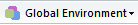 and you should see the list of lubridate’s functions.)
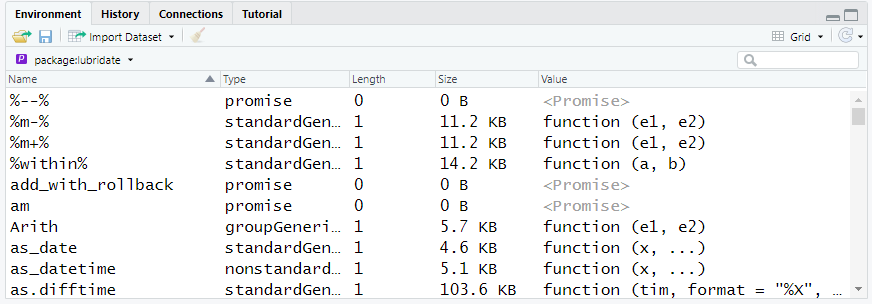
Figure 12.1: The lubridate functions live in the lubridate environment.
So . . . a package is a set of functions. But there’s more . . .
We can learn more about a package by using the packageDescription function:
## Type: Package
## Package: lubridate
## Title: Make Dealing with Dates a Little Easier
## Version: 1.7.9
## Authors@R: c(person(given = "Vitalie", family = "Spinu", role = c("aut", "cre"), email = "spinuvit@gmail.com"), person(given =
##                "Garrett", family = "Grolemund", role = "aut"), person(given = "Hadley", family = "Wickham", role = "aut"),
##                person(given = "Ian", family = "Lyttle", role = "ctb"), person(given = "Imanuel", family = "Costigan", role = "ctb"),
##                person(given = "Jason", family = "Law", role = "ctb"), person(given = "Doug", family = "Mitarotonda", role = "ctb"),
##                person(given = "Joseph", family = "Larmarange", role = "ctb"), person(given = "Jonathan", family = "Boiser", role =
##                "ctb"), person(given = "Chel Hee", family = "Lee", role = "ctb"))
## Maintainer: Vitalie Spinu <spinuvit@gmail.com>
## Description: Functions to work with date-times and time-spans: fast and user friendly parsing of date-time data, extraction and
##                updating of components of a date-time (years, months, days, hours, minutes, and seconds), algebraic manipulation on
##                date-time and time-span objects. The 'lubridate' package has a consistent and memorable syntax that makes working with
##                dates easy and fun.  Parts of the 'CCTZ' source code, released under the Apache 2.0 License, are included in this
##                package. See <https://github.com/google/cctz> for more details.
## License: GPL (>= 2)
## URL: http://lubridate.tidyverse.org, https://github.com/tidyverse/lubridate
## BugReports: https://github.com/tidyverse/lubridate/issues
## Depends: methods, R (>= 3.2)
## Imports: generics, Rcpp (>= 0.12.13)
## Suggests: covr, knitr, testthat (>= 2.1.0), vctrs (>= 0.3.0)
## Enhances: chron, timeDate, tis, zoo
## LinkingTo: Rcpp
## VignetteBuilder: knitr
## Encoding: UTF-8
## LazyData: true
## RoxygenNote: 7.1.0
## SystemRequirements: A system with zoneinfo data (e.g. /usr/share/zoneinfo) as well as a recent-enough C++11 compiler (such as g++-4.8
##                or later). On Windows the zoneinfo included with R is used.
## Collate: 'Dates.r' 'POSIXt.r' 'RcppExports.R' 'util.r' 'parse.r' 'timespans.r' 'intervals.r' 'difftimes.r' 'durations.r' 'periods.r'
##                .....
## NeedsCompilation: yes
## Packaged: 2020-06-03 11:12:59 UTC; vspinu
## Author: Vitalie Spinu [aut, cre], Garrett Grolemund [aut], Hadley Wickham [aut], Ian Lyttle [ctb], Imanuel Costigan [ctb], Jason Law
##                [ctb], Doug Mitarotonda [ctb], Joseph Larmarange [ctb], Jonathan Boiser [ctb], Chel Hee Lee [ctb]
## Repository: CRAN
## Date/Publication: 2020-06-08 15:40:02 UTC
## Built: R 4.0.2; x86_64-w64-mingw32; 2020-07-16 21:02:47 UTC; windows
##
## -- File: C:/RSiteLibrary/lubridate/Meta/package.rds
This output is generated from the package’s DESCRIPTION file. Soon you’ll be producing a DESCRIPTION file too! Not to worry, though, as all of this will be easy to do in the package development process.
But there’s more. Let’s dig a bit further with assistance of the help function.
You should see that the Help tab is enabled, showing the documentation for lubridate. (Alternatively, if you use RStudio, this page can be displayed by clicking on a package name in the “Packages” tab.)
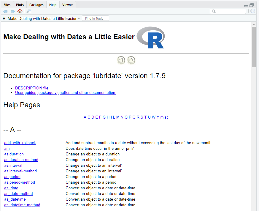
Figure 12.2: lubridate’s package documentation.
This file is split into two parts: Documentation and Help Pages.
Under the Documentation section, you see links to the DESCRIPTION file, User guides, package vignettes, and possibly a NEWS file.
Click on the DESCRIPTION file link and you should see the same information returned by the packageDescription function.
Click on the “User guides, package vignettes and other documentation” link and you should be able to navigate to lubridate’s vignette, which is a user-friendly tutorial. You can also use the vignette function to quickly pull the vignettes up for any package that has provided one::
Figure 12.3: lubridate’s vignette.
So . . . packages contain vignettes and other documentation. But there’s more . . .
The Help Pages section includes the package functions, listed alphabetically. Each function can have a helpfile, providing guidance to user’s about each function. By now, you’ve had a lot of experience using helpfiles!
Let’s find out where lubridate is actually stored on your computer.
PC users: In a previous chapter, we created a site library called “RSiteLibrary” on our C drive. When you installed lubridate, you downloaded the files into the site library directory.
Mac and Linux users: If you are on a Mac, you probably have only one library.
We can determine where exactly your R libraries are located on your machine with the .libPaths function:
## [1] "C:/RSiteLibrary" "C:/Program Files/R/R-4.0.2/library"You can see that we have two libraries (we’re on a PC), one holds the packages that come with “base” R and the second holds packages that we download elsewhere. Our site library is stored on our C drive in a folder called RSiteLibrary.
Mac users: the call to .libPaths probably returns something like this:
/Library/Frameworks/R.framework/Versions/4.0/Resources/libraryRegardless of what OS you use, for package creation, it is critical that you can write to your site library.
Now that you know where R stores your packages, navigate to site library folder, and open up the folder called lubridate. You can see several folders here, plus several files. These, collectively, make up the package.
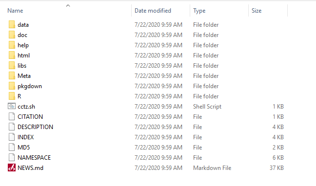
Figure 12.4: The lubridate package is downloaded as a set of directories and files, each storing specific information.
Look specifically for the folders R and help. The folder labeled R holds the package’s R functions. Wild! The folder labeled help stores the packages helpfile documentation. Double wild!! Now look for the files called DESCRIPTION and NAMESPACE. The DESCRIPTION file is the same file you viewed with the packageDescription function. The NAMESPACE file is required in order for your package to seamlessly work with other R packages . . . more on this later.
Go ahead and peer into these folders (but don’t change anything!). It’s very instructive to see what’s included in each file (you can use RStudio or some other text editor to view some files).
With all of these components, it’s no wonder why creating a package may feel overwhelming. However, you can create a bare-bones package that includes just functions, help pages, and a documentation file. And RStudio has several tools that make this process so easy that you’ll be storing collections of your homemade functions within packages in no time.
12.1 Load Required Packages and Programs
The RStudio helpfiles indicate that there are two main prerequisites for building R packages:
- GNU software development tools including a C/C++ compiler; and
- LaTeX for building R manuals and vignettes.

Figure 12.5: You must install some required software to create a package in R.
Before you go further, read this article on the RStudio help page and make sure you have the necessary tools for package development. This step involves installing new software onto your computer, and checking to make sure you’ve done it correctly. You may need to run R in administrator mode.
Assuming you are ready to go, let’s load the two packages designed to facilitate package development.
The devtools package contains many functions for building packages. Remember, everything R does is done via a function. Several of RStudio’s package development buttons run one or more functions from devtools.
The roxygen2 package allows you to quickly generate R documentation (Rd) files (help files…you know, all of the help files that you have been reading throughout the Fledgling chapters).
Finally, we are ready to begin.
12.2 Create your package directory
In R Studio, you create a package directory by going to File | New Project | New Directory | R Package.
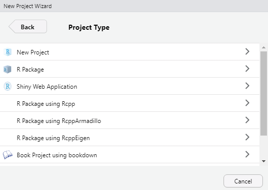
Figure 12.6: Create a new package as new project in RStudio.
After clicking on the R Package option, you identify your package name and directory by entering information into the dialogue box. Packages are projects in their own right, and should be stored in a unique directory that is not part of another R project. This directory should NOT be part of your site library! We repeat: This directory should NOT be part of your site library!
Here, we will create a new package called TTestimators in our C drive in a new directory called Rpackages.
We’ll add our sak and index functions right away. Click the Add button and navigate to your sak.R function, which is called a ‘source file’ because it will be sourced when the package is loaded. The click the Add button again and navigate to your index.R file. If you do not have any functions yet, you can skip this step (although you really should have completed Chapter 11 before starting on this chapter!). Again, make sure your project is not a subdirectory of another R project!
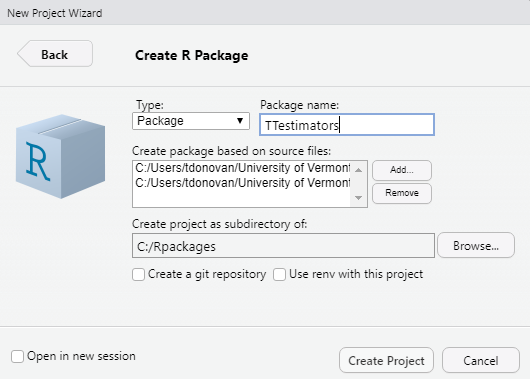
Figure 12.7: The Create R Package wizard will create a new R project that includes the ‘shell’ of a package.
Click the Create Project button.
RStudio should restart and open your new project. If not, close RStudio, navigate to the folder called TTestimators, and open the file called TTestimators.Rproj. Do this now!
If you look in this directory, you should see two folders (man and R) and two files (DESCRIPTION and NAMESPACE). You may or may not have the file .Rbuildignore (depending on whether you have file versioning software on your computer).
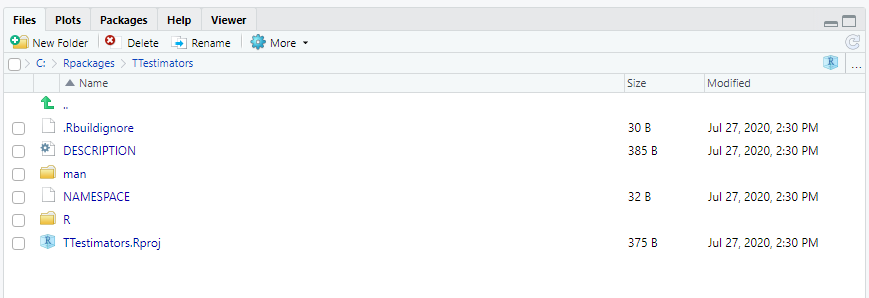
Figure 12.8: The package file structure.
Notice that this list is pretty scanty compared to the folders and files in lubridate. What you are looking at is the minimal requirements for package creation in R.
Let’s work through these one at a time.
First, the file TTestimators.Rproj is your R project file, which is the file you should open when you want to work on your package.
The NAMESPACE file is used to specify other packages that your package depends on. The default NAMESPACE file looks like this:
exportPattern("^[[:alpha:]]+")This is the file where you add “package dependencies” – packages that your package needs to run. For example, if our package required the lubridate package to properly run, we would add the line import(lubridate) to this file, like this:
import(lubridate)
exportPattern("^[[:alpha:]]+")
Our TTestimators package does not have any imports, so we can leave the default as it is.
- The DESCRIPTION file gives a description of the package (we looked at lubridate’s DESCRIPTION FILE, and will need to create our own file for the TTestimators package . . . we’ll do that soon).
In addition to the NAMESPACE and DESCRIPTION files, two directories (folders) were created. The helpfiles will be stored in the folder called man, which is short for manual. And the R functions will be stored in the folder called R.
12.3 Add functions
Our TTestimators package will contain the sak and index functions we built in the last chapter. It will also include a sample dataset so that users can run demos and examples.
Open up the R folder in your project, and if you included your sak.R and index.R files, you should see them in this folder. If you did not include any source files when you created the package skeleton, you will see a file called TTestimators.R. This file is empty and was created by default so it can be used for documentation or functions.
The R folder will hold all of your package functions, which are .R scripts. Our package will contain just two functions, but as you’ve seen, packages are collections of functions.
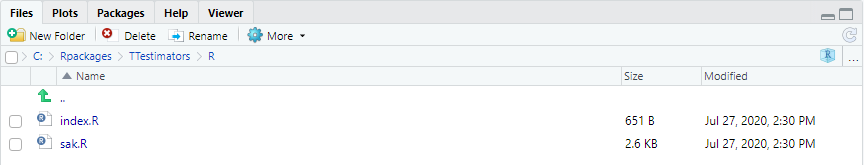
Figure 12.9: The R folder contains the actual R functions.
Some people will create a separate .R file for each and every function as a way of keeping files tidy. Others will cram all functions into a single .R file, such as TTestimators.R. And still others will create a few .R files that contain groupings of functions. We favor the one-file-per-function approach, but it’s up to you how you want to organize files.
If you have not done this already, copy the sak.R and index.R files into the R directory in our TTestimators project. Do this now! You can do this in R with the
file.copyfunction if you don’t want to use your mouse. Remember, however, that you are now in the package project, not your R_for_Fledglings project! You’ll need to include the full file path to get things right. Remember thatchoose.dircan help you find the file path.
12.4 Add Datasets
In addition to R functions, many R packages come with built-in datasets to help a user learn the package quickly. Datasets can be .tab, .txt, .csv, or .RData files, and must be stored in a new folder called data. You’ve probably noticed that this folder was NOT automatically created for you, so we need to create one now (either by clicking the  button in the Files tab, or with code as shown) Here, we will use the absolute (full) file paths. If your folder locations differ, you will need to adjust the code below!
# create a new directory called data within the package folder.
dir.create("C:/RPackages/TTestimators/data")
Remember the TauntaunData.RDS file we worked with in previous chapters? This the final version of the harvested dataset, cleaned of mistakes and merged with hunter information. This should be located in your R_for_Fledglings project in a folder called ‘datasets’. We would like to include this dataset in our R package. However, R packages cannot contain RDS files in the data folder. So, we’ll read in the TauntaunData.RDS file (from our Fledglings project), and save it as TauntaunHarvest.RData to the “data” folder in our TTestimators package project.
Here, we’ll use full file path to the RDS file that work on our machine. You will need to make the correct adjustments!
# read in the TauntaunData.RDS file
TauntaunHarvest <- readRDS("C:/Users/tdonovan/University of Vermont/Spreadsheet Project - General/R Training/Fledglings/datasets/TauntaunData.RDS")

# write this as a csv file to the package "data" folder
save(TauntaunHarvest, file = "C:/RPackages/TTestimators/data/TauntaunHarvest.RData" )
At this point, we now have two .R files in our R folder, and one .RData file in the data folder. The next step is to add documentation.
12.5 Add documentation
12.5.1 The DESCRIPTION File
Documentation includes writing the helpfiles and filling in the DESCRIPTION file. Let’s start with the DESCRIPTION file, which is a snap. Open this file in RStudio, and the you should see the following:
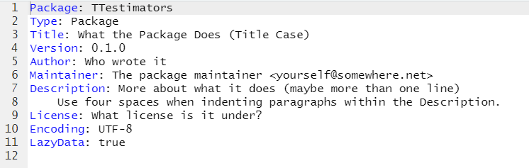
Figure 12.10: TTestimators’ description file.
Edit this file to provide a good description of your package. Remember, though, that this is what users will see if they use the packageDescription function. See Hadley Wickham’s book on R packages writing a well-crafted DESCRIPTION file.
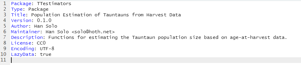
Figure 12.11: TTestimators’ description file.
This file is pretty self-explanatory. The exception is the ‘License’ option, where you specify the conditions of use. You will probably select GPL-2 (free distribution and modification; free as in free speech), as that is what most people select, but see http://www.r-project.org/Licenses/ for more information.
If you plan to check your package (e.g. to submit to CRAN), you will need to specify a minimum R version of 2.10.0 to ensure users will have access to the data folder.
- Add a field Depends: R (>= 3.5.0) to the DESCRIPTION file to take care of this.
12.5.2 Rd files
Next, you need to document the functions in your package. These are called .Rd files, which stands for “R Documentation”.
As Hillary Parker explains:
“This always seemed like the most intimidating step to me. I’m here to tell you - it’s super quick. The package roxygen2 that makes everything amazing and simple. The way it works is that you add special comments to the beginning of each function, that will later be compiled into the correct format for package documentation. The details can be found in the roxygen2 documentation.”
In the roxygen2 documentation, we read:
“Documentation is one of the most important aspects of good code. Without it, users won’t know how to use your package, and are unlikely to do so. Documentation is also useful for you in the future (so you remember what the heck you were thinking!), and for other developers working on your package. The goal of roxygen2 is to make documenting your code as easy as possible.”
12.5.2.1 Documenting the sak function
Now we’ll add documentation for the sak function. The “special comments” that Hillary referred to can be seen in the code block below, which is inserted ABOVE the sak function code.
Copy this code now, and paste ABOVE your sak function in sak.R. Be sure to paste this into the sak.R file that was copied into your TTestimators package’s R directory, not your original sak.R file from Chapter 11!. Also, do not copy the actual
sakfunction code below . . . it is displayed only for orientation. Each line should begin with #'. Oh, one more thing: Make sure that your pasted code lines up with the left-hand margin in your script!
#' @title Sex-Age-Kill Estimator
#' @description This function estimates the population size of a harvested species immediately
#' before the harvest was initiated based on the method proposed by Eberhardt.
#' @param harvest_data A dataframe containing harvested animals, where each row of data is a
#' single animal. See Details for more information.  The harvest dataframe must have a column
#' called "year".
#' @param year  The year of the analysis.  The function will subset the harvest_data to include
#' records for the year of interest.
#' @param proportion_mortality_harvest The proportion of the total annual mortality for breeding
#' males that is due to harvest.  For example, if  60\% of the total annual mortality is due to
#' harvest mortality and 40\% due to other mortality factors, then  set
#' proportion_mortality_harvest to 0.6.
#' @param offspring_per_female  The per capita birth rate for breeding females.  This is a
#' population level rate. The default value is 2.
#' @concept sak
#' @concept sex-age-kill
#' @keywords model
#' @author Han Solo
#' @details The harvest dataset should be a dataframe with one row per harvested Tauntaun.  This
#' dataframe must include a column called "sex", where the sex of each individual is listed as
#' "m", "f", or "u" (for unknown), and a column called "year", which indicates the year of harvest
#' as integers (e.g., 1901, 1902, etc).  Additionally, a column called "age" should include the
#' age of individuals as an integer (e.g., 0, 1, 2, 3, ...).
#' @export
#' @examples
#' # load in the built-in dataset
#' data(TauntaunHarvest)
#'
#' # run the function to analyze the 1901 data
#' results <- sak(TauntaunHarvest,
#'                year = 1901,
#'                proportion_mortality_harvest = 0.5,
#'                offspring_per_female = 2.0)


sak <- function(harvest_data,
                year,
                proportion_mortality_harvest,
                offspring_per_female = 2){
This is how you build your helpfile. The helpfile documentation precedes the function’s code.
After pasting the documentation in, save your sak.R file. The helpfile content is added prior to the function itself. Keeping the help files associated with the function makes it easier update the documentation if/when the function is updated.
Each comment begin with a hashtag # sign, followed by a single quote '. Then, after a space, you see several tags, such as param, keywords, export, and examples, all beginning with an @ symbol. These tags identify a specific section of the help page. Notice that #' is followed by a space, and then the tag value, which is followed by another space, and then a description.
Look through these special comments now!
The special “tags” have a specific syntax, but there is an easy way to remember them. As you start creating a new comment, after you enter @, press the tab key and you should see a list of potential options.
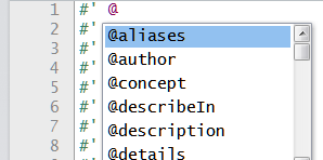
Figure 12.12: Use the tab key to see a list of tags.
Here, you may see the “old friends” that you’ve seen in various helpfiles, such as author, description, details, examples, etc.
Of these, a few should always be include in your helpfile:
- @title - the name of the function
- @description - a brief description of the function
- @param - the function’s arguments, along with a short description. Each argument is entered as a separate tag.
- @export - must be included if the function’s helpfile is to be written. If this line is missing, the function’s helpfile will not be written.
- @examples - examples of how to use the function. As we’ve seen, this often involves creating a little example problem from scratch.
- @keywords - to help a user find your function. Each keyword is entered separately.
- @details - additional information about the function that goes beyond the description tag.
When writing the definitions for a comment, you’ll need to pay attention to symbols that may have multiple meanings. For example, take a look at the the line beginning with #' @param proportion_mortality_harvest. In this line, we define the argument to the sak function called proportion_mortality_harvest, and then define what this argument means. Look for the section that says “if 60\% of the total annual mortality . . .”. What’s with the backslash in front of the percent symbol? Ultimately, these comments will be translated into LaTeX, and the comment character in LaTeX is a percent % sign. So, just writing 60% will cause some problems. If you want to print a percent sign in your comment, you need to escape each % character with a backslash \.
Keywords are also important because they guide the CRAN server searches. To choose keywords, you will want to consult the list of standard keywords used by R functions. The list of standard keywords can be found in the R_HOME/doc/KEYWORDS file. You can view this file in your R console:
## GROUPED Keywords
## ----------------
##
## Graphics
## 	aplot		&	Add to Existing Plot / internal plot
## 	dplot		&	Computations Related to Plotting
## 	hplot		&	High-Level Plots
## 	iplot		&	Interacting with Plots
## 	color		&	Color, Palettes etc
## 	dynamic		&	Dynamic Graphics
## 	device		&	Graphical Devices
##
## Basics
## 	sysdata		&	Basic System Variables		[!= S]
## 	datasets	&	Datasets available by data(.)	[!= S]
## 	data		&	Environments, Scoping, Packages [~= S]
## 	manip		&	Data Manipulation
## 	attribute	&	Data Attributes
## 	classes		&	Data Types (not OO)
## 	    & character	&	Character Data ("String") Operations
## 	    & complex	&	Complex Numbers
## 	    & category	&	Categorical Data
## 	    & NA	&	Missing Values			[!= S]
## 	list		&	Lists
## 	chron		&	Dates and Times
## 	package		&	Package Summaries
##
## Mathematics
## 	array		&	Matrices and Arrays
## 	      & algebra &	Linear Algebra
## 	arith		&	Basic Arithmetic and Sorting	[!= S]
## 	math		&	Mathematical Calculus etc.	[!= S]
## 	logic		&	Logical Operators
## 	optimize	&	Optimization
## 	symbolmath	&	"Symbolic Math", as polynomials, fractions
## 	graphs		&	Graphs, (not graphics), e.g. dendrograms
##
## Programming, Input/Ouput, and Miscellaneous
##
## 	programming	&	Programming
## 	     & interface&	Interfaces to Other Languages
## 	IO		&	Input/output
## 	     & file	&	Files
## 	     & connection&	Connections
## 	     & database	&	Interfaces to databases
## 	iteration	&	Looping and Iteration
## 	methods		&	Methods and Generic Functions
## 	print		&	Printing
## 	error		&	Error Handling
##
## 	environment	&	Session Environment
## 	internal	&	Internal Objects (not part of API)
## 	utilities	&	Utilities
## 	misc		&	Miscellaneous
## 	documentation	&	Documentation
## 	debugging	&	Debugging Tools
##
## Statistics
##
## 	datagen		&	Functions for generating data sets
## 	distribution	&	Probability Distributions and Random Numbers
## 	univar		&	simple univariate statistics  [!= S]
## 	htest		&	Statistical Inference
## 	models		&	Statistical Models
## 	    & regression&	Regression
## 	    & &nonlinear&	Non-linear Regression (only?)
## 	robust		&	Robust/Resistant Techniques
## 	design		&	Designed Experiments
## 	multivariate	&	Multivariate Techniques
## 	ts		&	Time Series
## 	survival	&	Survival Analysis
## 	nonparametric	&	Nonparametric Statistics [w/o 'smooth']
## 	smooth		&	Curve (and Surface) Smoothing
## 	     & loess	&	Loess Objects
## 	cluster		&	Clustering
## 	tree		&	Regression and Classification Trees
## 	survey		&	Complex survey samples
##
##
## MASS (2, 1997)
## --------------
##
## add the following keywords :
##
## 	classif		&	Classification	['class' package]
## 	spatial		&	Spatial Statistics ['spatial' package]
## 	neural		&	Neural Networks ['nnet'	 package]
For our sak function, we’ve added the keyword models because the function models the living population size, but note that they keyword, models, typically refers to statistical models.
If you’d like to use non-standard keywords, the Writing R Extensions guide tells use to use the tag, @concept.
As you are well aware, the @examples are super important for your user. Our example included the use of our built-in dataset called ‘TauntaunHarvest’ (which is the csv file that you added to the “data” folder. When the package is loaded, this csv file can be loaded to R with the data function. You can add as many different examples as you think necessary. These must be free of error, and able to be executed by a user by copying and pasting the code into the console, or by running the example function. We’ll test this later (and add more examples).
In writing your helpfiles, it’s worth repeating these little ditties from Chapter 11 (Writing Functions):
“Essentially style resembles good manners. It comes of endeavouring to understand others, of thinking for them rather than for yourself - or thinking, that is, with the heart as well as the head.” - Sir Aurthur Quiller-Couch “And how is clarity to be achieved? Mainly by taking trouble; and by writing to serve people rather than to impress them.” - F. L. Lucas
We’ve all read helpfiles that, well, aren’t very helpful. This is YOUR chance to write the best documentation the world has ever seen! You can find more information in the roxygen2 vignette.
12.5.3 Process your documentation
Now you need to create the documentation from your annotations earlier. You’ve already done the “hard” work in the previous step. This step is simple, and uses the document function from devtools. Run the following code:
You’re done! The document function is used to convert the special comments you just added into .Rd files (short for R documentation files), which are then added to the man folder (short for manual) in your package directory. Have a look!
Figure 12.13: Use the tab key to see a list of tags.
If you open the sak.Rd file (navigate to it in RStudio), you should see something like this:
Figure 12.14: An Rd file is coded with LaTex.
Yowsa! Roxygen2 converted your tags into this LaTex document (which you could have written by hand). But, it’s much easier to use the roxygen2 shortcuts, don’t you agree? Notice the warning at the top of the page: Generated by roxygen2: do not edit by hand.
With your sak.Rd file open, look at the top of this file for toolbar that looks like this 
Click on the Preview button, and you’ll see what the help page will look like to a future user of your sak function.
Figure 12.15: A preview of your sak helpfile.
How does your helpfile look? It should look like one of R’s standard helpfiles that you have grown to know and love (at least a little!).
Hadley Wickham, one of the authors of the roxygen2, describes writing documentation as a four-step process:
- Add roxygen comments to your .R files.
- Run devtools::document() (or press Cmd + Shift + D in RStudio) to convert roxygen comments to .Rd files.
- Preview documentation with the Preview button (or with
?orhelpafter the package is loaded). - Rinse and repeat until the documentation looks the way you want.
Exercise: 1. Add another example to the @examples section, and include an example where the user passes in a vector of values for proportion_mortality_harvest. You can simply press Return after the first example, and the #' prompt should be diplayed in the next line. Press Return again for another line (again the #' prompt should appear), and start typing your new example. Make sure to include comments in your examples to explain to your function user what the code is doing! 2. Add another example to the @examples section, and include an example where the user passes in a vector of values for years. Make sure to include comments in your examples to explain to your function user what the code is doing! 3. Create documentation for the index function, including at least 2 examples.
12.5.4 Documenting the TauntaunHarvest Dataset
Our dataset also needs to be documented, and dataset documentation is a bit different than function documentation. While there are ways to use roxygen comments to document a dataset, here, we’ll take this opportunity to show you how to create an .Rd file directly.
Go to File | New file | R documentation, and fill in the dialogue box, indicating that the Topic is TauntaunHarvest and that the documentation is for a dataset.
Figure 12.16: The dataset documentation template.
Press OK, and you should see a new .Rd file, with syntax that looks like the syntax that roxygen2 generated. This is a template that is meant to be edited.
\name{TauntaunHarvest}
\alias{TauntaunHarvest}
\docType{data}
\title{
%%   ~~ data name/kind ... ~~
}
\description{
%%  ~~ A concise (1-5 lines) description of the dataset. ~~
}
\usage{data("TauntaunHarvest")}
\format{
  A data frame with 0 observations on the following 2 variables.
  \describe{
    \item{\code{x}}{a numeric vector}
    \item{\code{y}}{a numeric vector}
  }
}
\details{
%%  ~~ If necessary, more details than the __description__ above ~~
}
\source{
%%  ~~ reference to a publication or URL from which the data were obtained ~~
}
\references{
%%  ~~ possibly secondary sources and usages ~~
}
\examples{
data(TauntaunHarvest)
## maybe str(TauntaunHarvest) ; plot(TauntaunHarvest) ...
}
\keyword{datasets}
Can you find the tags? They begin with a backslash. Here, you see the use of @docType (set to data). The idea here is that you fill in the template entries as best you can. The sections that begin with %% are meant to be edited. For instance, you can delete the line %% ~~ data name/kind … ~~ and fill in the title for this help page.
The section called format is a critical one - here you describe the dataset and describe each and every column in the dataset. We’ve modified this file as shown below:We’ve edited this file as follows:
\name{TauntaunHarvest}
\alias{TauntaunHarvest}
\docType{data}
\title{Example Tauntaun Harvest Dataset
}
\description{This dataset was simulated and edited throughout chapters of the ebook, R for Fledglings. Each row of data describes a single harvested tauntaun.
}
\usage{data(TauntaunHarvest)}
\format{
  A data frame with XX observations on the following 19 variables.
  \describe{
    \item{\code{hunter.id }}{a numeric vector}
    \item{\code{age}}{a numeric vector containing integer values of age}
    \item{\code{sex}}{a factor with 2 levels}
    \item{\code{individual}}{a numeric vector uniquely identifying each animal}
    \item{\code{species}}{a character vector identifying the species}
    \item{\code{date}}{a date vector indicating the date of harvest}
    \item{\code{town}}{a factor indicating the town of harvest}
    \item{\code{length}}{a numeric vector giving length of the tauntaun}
    \item{\code{weight}}{a numeric vector giving the weight of the tauntaun}
    \item{\code{method}}{a factor indicating the method of harvest}
    \item{\code{color}}{a factor indicating the fur color}
    \item{\code{fur}}{a factor indicating the length of fur}
    \item{\code{month}}{a numeric vector between 1 and 12 indicating the month of harvest}
    \item{\code{year}}{a numeric vector indicating year of harvest}
    \item{\code{julian}}{a numeric vector indicating the julian date of the harvest}
    \item{\code{day.of.season}}{a numeric vector indicating the day within the harvest season in which the animal was harvested}
    \item{\code{sex.hunter}}{a factor indicating the sex of the hunter}
    \item{\code{resident}}{a logical vector indicating whether the hunter was a resident or not}
    \item{\code{count}}{a numeric vector with values set to 1}
  }
}
\details{Tauntauns are omnivorous reptomammals indigenous to the icy planet of Hoth. Tauntauns
were first observed in the USA in the late 1700's and they have dispersed to most of the cold
-winter states. Tauntauns were first identified in Vermont in 1848 and the Department has been
tracking the population of Vermont's tauntaun through harvest records since 1901.
}
\source{http://www.uvm.edu/~tdonovan/RforFledglings/}

\examples{
data(TauntaunHarvest)
head(TauntaunHarvest)
str(TauntaunHarvest)
}
\keyword{datasets}
Notice that our examples make use of the data, head, and str functions.
Save this file as TauntaunHarvest.Rd (save it directly in the man folder). Now, use the Preview button to see how it will look.
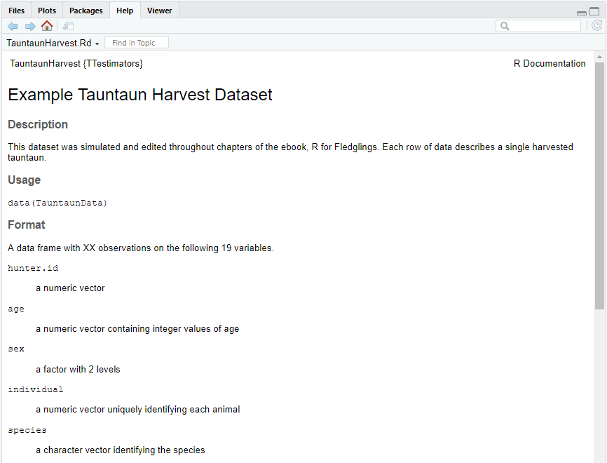
Figure 12.17: The built-in TauntaunHarvest helpfile.
Not bad! Of course, rinse and repeat cycles are critical to get it just right.
Oh! One more thing! Add the following line to your DESCRIPTION file if it is not there (with no spaces between lines):
LazyData: TRUEThis will allow a user to load the dataset into R’s global environment when the package is loaded.
12.5.5 Documenting the TTestimators-package
There’s one more .Rd file we should create/edit, and that is the .Rd file that automatically created when you created the package project. In the man folder, look for the file called TTestimators-package, and open it. This is another template, meant to be edited. This .Rd file stores your package “metadata”. If this file is not present, just go to File | New File | R Documentation, and select “Empty Topic” for the template:
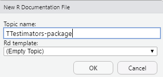
Figure 12.18: lubridate’s helpfile.
Before we go further, what is this file for? The crux of this .Rd file is to provide an overview of your package. You can read more about it here. As Hadley Wickham writes:
“As well as documenting every exported object in the package, you should also document the package itself. Relatively few packages provide package documentation, but it’s an extremely useful tool for users, because instead of just listing functions like help(package = pkgname) it organises them and shows the user where to get started . . . Package documentation should describe the overall purpose of the package and point to the most important functions. This file is for human reading, so pick the most important elements of your package.”
Copy the code below in this file, and save it as TTestimators-package.Rd.
\name{TTestimators-package}
\alias{TTestimators-package}
\alias{TTestimators}
\docType{package}
\title{
Functions for estimating population size from harvested animals.
}
\description{
Many species of animals are harvested during a discrete harvest season.  A suite of estimation
methods are available that can estimate the size of the living population (immediately before
the harvest) from the (dead) animals that have been harvested. Each method has unique assumptions
which must be checked and verified before using a particular analysis.
}
\details{
\tabular{ll}{
Package: \tab estimators\cr
Type: \tab Package\cr
Version: \tab 1.0\cr
Date: \tab 2014-12-09\cr
License: \tab GPL-2 | GPL-3 \cr
}
Each function requires specific inputs, one of which is the harvested dataset.  The assumption is that each line of data in the harvested dataset is a record for a single animal.
}
\author{
Han Solo
Maintainer: Who to complain to <solo@hoth.net>
}
\keyword{ package }
\examples{
data(TauntaunHarvest)
sak(TauntaunHarvest,
                year = 1901,
                proportion_mortality_harvest = 0.5,
                offspring_per_female = 2)
}
When you run document again, this file will be listed in the package’s documentation. We’ll look for it after we “build” our package.
12.6 Vignettes
A vignette is “a small, graceful literary sketch”. Although not required, they provide an opportunity for package creators to offer more verbose and user-friendly documentation for their package. In this section, we’ll describe vignettes, although we won’t be writing one for our estimators package.
There are few rules guiding what should be in the content of a vignette, or how many vignettes a package can have. However, packages that are submitted to CRAN have a recommended package size. Because vignettes are a source of extra bulk, if your package exceeds the size limit, package authors may strip out the vignettes in order to meet CRAN’s target size. However, package users will really appreciate a well-crafted vignette, and we encourage you to produce them! Vignettes typically provide additional examples of package use, a rationale for a function’s design, or any information that didn’t fit the standard package documentation templates.
If you’d like to include a vignette(s) to your package, they must be stored in a new directory called vignettes.
Vignettes can be easily created with R Markdown (as we did in Chapter 10). R Markdown can be used to write documents with R code embedded in them, and when knitted they produce HTML or PDF documents that merge text, R code, and R output. When an R Markdown vignette is included in a package, the .Rmd file should be placed in the ‘vignettes’ directory.
If you create your vignette as an R markdown file, two things need to be done from the package-building perspective. First, the file’s metadata needs to indicate that it is a vignette. You can use RStudio to help you create a new vignette in R markdown. To to File | New File | R Markdown | From Template | Package Vignette:

Figure 12.19: Use the Package Vignette Template to create a vignette (or two) for your package.
Look at the metadata in this file. It contains new information that indicates the file is a vignette. Specifically, notice the following lines of code to the .Rmd metadata section:
---
title: "Vignette Title"
author: "Vignette Author"
date: "2021-01-06"
output: rmarkdown::html_vignette
vignette: >
  %\VignetteIndexEntry{Vignette Title}
  %\VignetteEngine{knitr::rmarkdown}
  %\VignetteEncoding{UTF-8}
---
This file, when knit, will produce an html vignette that can be added to the vignette folder.
- Second, you must add an additional line to the DESCRIPTION file:
VignetteBuilder: knitrWe won’t spend time building a vignette for the TTestimators package, but make sure to review Chapter 10 if you plan to include vignettes with your package. A well-written vignette is super helpful for your users.
12.7 Build!
To work with packages in RStudio, you use the Build pane, which includes a variety of tools for building and testing packages.
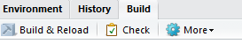
While iteratively developing a package in RStudio, you typically use the Build and Reload button  to re-build the package and reload it in a fresh R session.
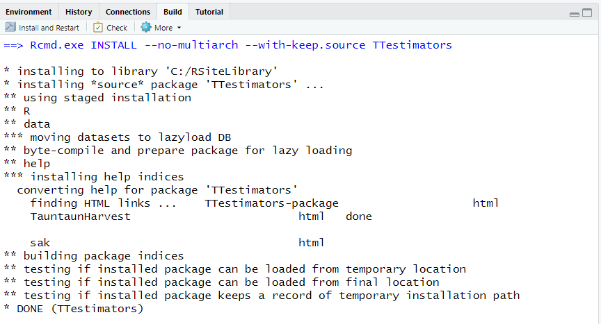
Figure 12.20: The Build Pane shows the steps of the package building process.
According to the RStudio helpfile, the Build and Reload command performs several steps in sequence to ensure a clean and correct result:
- Unloads any existing version of the package (including shared libraries if necessary).
- Builds and installs the package using R CMD INSTALL.
- Restarts the underlying R session to ensure a clean environment for re-loading the package.
- Reloads the package in the new R session by executing the library function.
After pressing the Build & Reload button, you should see that the package has been built, and the console shows the following:
Restarting R session...

> library(TTestimators)
>
In the Build Pane, you will see a list of tasks that has been executed. Hopefully you were able to get this to run. If not, the output displays errors and warnings, and your job is to now fix them. Pay attention to any file names and line numbers displayed in this output – this tells you where to start your hunt.
At this point, we have a “real, live, functioning R package”. The package is located in your site library, just as if you had downloaded it from CRAN. Let’s check (assuming your site library is located at “C:/RSiteLibrary”):
# verify that the estimators directory is in your RSiteLibrary folder
file.exists("C:/RSiteLibrary/TTestimators")
## [1] TRUENow that we have a real package, let’s try the following:
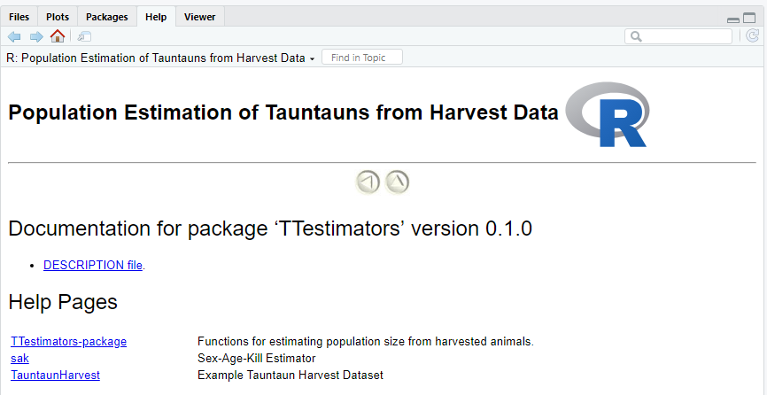
Figure 12.21: TTestimators package documentation.
If all goes well, the following code should work. Try it out for yourself!
12.8 Iterate
The process of building a package is iterative. As Hillary Parker says:
“This is where the benefit of having the package pulled together really helps. You can flesh out the documentation as you use and share the package. You can add new functions the moment you write them, rather than waiting to see if you’ll reuse them. You can divide up the functions into new packages. The possibilities are endless!”
Each time you change the documentation, make sure to run document. And each time you change the actual code, make sure to re-build the package again. Remember, your built package is sent to your package library. When you run the library function, R is loading the package from that library, not from where your package project, TTestimators.
12.9 Checking Your Package
Even if your package successfully built, it doesn’t mean it is ready for the big-time. If you would like R to check your package structure, documentation, and function (by running the examples from the manual), you can run a check by clicking on the check button in the Build pane.
It is good practice to check your package if you plan to distribute it at all, and to fix any warnings or errors that are reported.
Do this now!
You will see a happy check mark next to items that pass, a W next to items that are warnings, and an ugly E for errors.
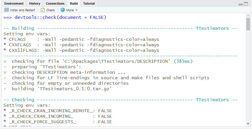
Figure 12.22: TTestimators code check.
For goodness sake, don’t blast through the messages that appear in the Build panel – R is telling you where the errors and warnings are, so make sure to slow down, take a deep breath, and work through the issues one at a time. Repeat the check until your package passes with no warnings or errors. We, ummm, had an issue with our build because we didn’t create the index Rd file. Ooops!
If you do encounter errors, fix them, then rebuild the package, and run the check again. Eventually you should see this happy result:
-- R CMD check results --------------------------------- TTestimators 0.1.0 ----
Duration: 19.4s

0 errors v | 0 warnings v | 0 notes v

R CMD check succeeded
Even if your package is only for your use, we recommending running the check until there are no errors.
12.10 Building for Distribution
If you plan to submit your package to CRAN, you will want to run the check as CRAN would run the check, which is more rigorous than a standard check. To check as CRAN you can open Tools | Project Options and select “Build Tools”.
In the box labeled “Check Package – R CMD check additional options” type “–as-cran” (no quotes) and click OK.
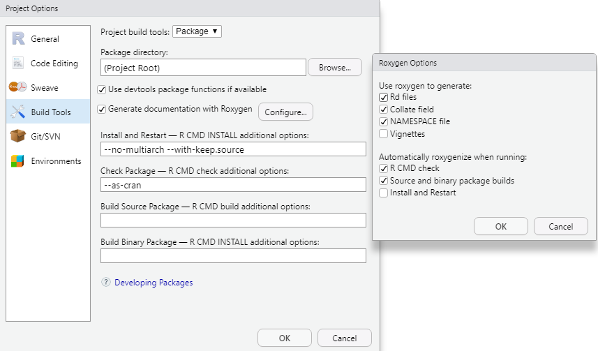
Figure 12.23: Set the project options to package, and then configure the roxygen.
Now return to your Build pane and press the check button, and you should observe that the check is more rigorous than previous checks, and any warnings, notes, and errors are sent to the file TTestimators.Rcheck/00check.log. To be accepted by CRAN, your package will need to pass this check with no errors or warnings, and notes are only allowed if your submission is accompanied by an explanation of why they could not be eliminated.
Once the package passes check, you can build the package, either by clicking the Build & Reload button in the Build pane (if you want just a local version, as we’ve done so far) or by selecting the More menu in the Build pane and choosing one of the Build options: Build Source Package or Build Binary Package.
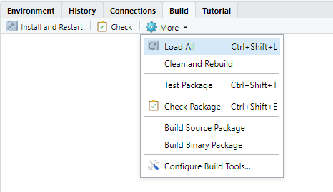
Figure 12.24: The More button shows additional tools for building the package.
For a CRAN contribution, you should select Build Source Package, which will create a tarball (e.g. estimators_1.0.tar.gz) in the parent directory. This is the file you submit to CRAN if you’d like broadly share your package. Once it passes through the CRAN server check farm, this tarball will appear in the package repository as the “Package source”. Linux users will be able to install this package source directly with the install.packages command, but Windows users typically install packages as a Windows-binary (a .zip file), and Mac OS users install as an OS X binary (a .tgz file). These alternate versions will be created by the CRAN maintainers over the course of the next 48 hours, and will eventually appear on the package page alongside the package source.
If you do not plan to contribute your package to CRAN but would still like to distribute it, you can select More | and then build the package in one of two ways (do both if your Tauntaun colleagues use different operating systems):
Build Binary Package. This will create a Windows binary (e.g. TTestimators_1.0.zip) in the parent directory,
Build Source Package. As previously described, this will create a tarball (e.g. TTestimators_1.0.tar.gz) in the parent directory.
At this point, you can send these files to your Tauntaun colleague. How will they load it? There are two ways.
First, they can use the Packages pane in RStudio. Click on the Install button, and when the dialogue box appears, select Install from Package Archive File, and have them navigate to the file you sent them.
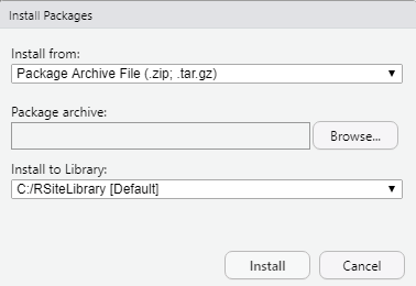
Figure 12.25: Installing a package from a local source.
Second, they can use the install.packages function, but enter it this way:
By invoking the choose.dir function, R brings up a window that will let a user browse to the package file directly.
12.11 Next Steps
Well done, fledglings! Hopefully you were able to get things running. We thank Hillary Parker for her wisdom when it comes to packages– start simple, and get through the whole process so you can see what’s what. Your homework is to now scan some of the documents that we mentioned early on. Happy reading!
We’re wrapping up our book, and you’ve come so very far in your R journey. In the next chapter, we will introduce the topic of simulations – we will show you how we created the virtual Tauntaun population that we introduced way back in Chapter 5. See you there!