Chapter 1 Introduction

We’ve been asked to provide a short introduction to R and its utility in natural resource management. In this short introduction, we can guarantee one thing: you won’t learn R in a few days. That would be like learning to speak French in a few days. To actually learn R, you need to practice . . . Michael Phelps didn’t win his Olympic medals without hours and hours of practice. However, in this short introduction, you can gain an appreciation for what R can do, be introduced to some key functions that you will likely use over and over again, and learn some strategies for creating scripts for automating your work. There are several excellent R books that provide much more information than this short introduction . . . R has a steep learning curve, and our hope is to cover some basics to get you over the initial hump.

Tip: To open hyperlinks in this book in a new window, try Ctrl+click (Windows) or command+click (Mac).

1.1 What is R?

Everything you want to know about R can be found at http://r-project.org/. From this site, we learn that:

“R is a system for statistical computation and graphics. It is a GNU project which is similar to the S language and environment which was developed at Bell Laboratories by John Chambers and colleagues. R can be considered as a different implementation of S…..R is available as Free Software under the terms of the Free Software Foundation’s GNU General Public License in source code form. It compiles and runs on a wide variety of UNIX platforms, Windows and MacOS.”

R was developed by Ross Ihaka and Robert Gentleman, and is described in the article, R: A Language for Data Analysis and Graphics. In that article, the authors indicate:

“We have named our language R– in part to acknowledge the influence of S and in part to celebrate our own efforts.”

So “R” stands for Robert and Ross.

When you download R, you download what is known as the “R core” program, or the “base R” program. This is the analysis engine and workhorse. But there’s more than just the core. While base R can perform a suite of basic analyses and mathematical functions, one of the main benefits of R is that it is highly extensible. This means that others can contribute to the functionality of R by developing “packages”. Think of a package like an add-on. The next two images are courtesy of Derek Ogle, author of a package called fishR. In the figure below, we see that packages are added to the R Core program.

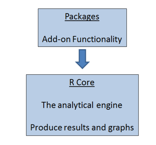
Figure 1.1: Base R + add-on packages.

Packages can be added onto your R program and can come from a variety of sources. Of these, the main source is often the Comprehensive R Archive Network (CRAN), where you can follow the “packages” link in the left menu and find a table of available packages. Thousands of packages are posted there, sorted by date of publication or sorted by name. Packages can be obtained from other repositories as well, such as R-Forge, GitHub, or dedicated GitLab sites, such as the USGS code repository. Additionally, you may develop your own package and store it on your local computer, as well as send your package to colleagues where they can load it on their machine. Regardless of the source, the packages are added to the base R program that is on your computer. We will review packages in greater depth in Chapter 3.

Together, the base R and packages permit a workflow that many people find very efficient. As outlined in the figure below, you open R and load any packages you need (light blue boxes). Then you send R your datasets, often in the form of external files such as a .txt, .csv., .xlsx, or other file (lower yellow box). You use a script editor, such as NotePad++, RStudio, or Tinn-R, to send commands to R (upper yellow box). In this book, we will use RStudio’s built-in script editor. R then analyzes the code and produces output. You’ll be able to store output as graphics, html documents, PDF files, and many other formats (upper red box). Finally, you can reproduce each and every step by creating a LaTex or Markdown document (lower red box), which lets you weave text with R. The document you are reading, for example, is a RMarkdown file. We’ll learn about each of these components throughout the Fledglings book.

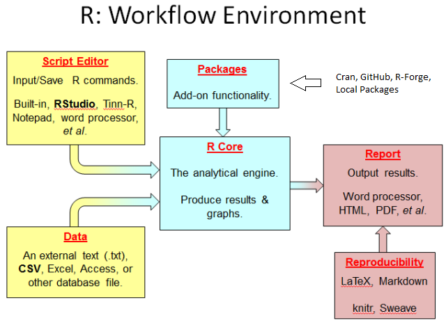
Figure 1.2: R workflow.

If you have not installed R yet, click here and install it now. If you have R on your computer, make sure that you have the most recent version.

1.2 What is RStudio?

RStudio is one of many script editors that you can use to interface with R. You type in commands into a script file (just a text file), and then send the commands from the script editor to R, where the code will be executed. RStudio can be found at http://www.rstudio.com/.

Install RStudio now if you haven’t already done so. If you already have RStudio on your machine, make sure you are running the latest version (go to Help | Check for Updates).

RStudio is much more than a script editor, however. Your code is entered into the Script editor (or source editor ) in the upper left hand pane. You’ll see this pane as soon as you start your first script in chapter 2! The entered code is then sent to the main R Console in the lower left pane, which is the analytical engine where the magic happens. A history of the commands you send to the R console is stored in the History pane in the upper right hand corner, along with what is called the R workspace. This workspace stores any objects you’ve created in R’s memory. In the lower right hand pane, RStudio provides a way to navigate to and organize files, view and save plots you create, install packages, and get help. In the next chapter, we’ll take a spin through RStudio in more detail.

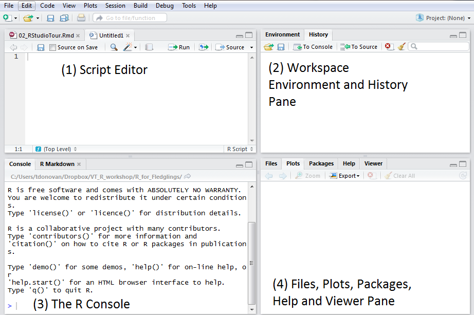
Figure 1.3: RStudio interface.

1.3 Project Goals

Our philosophy is that people learn best by doing, so throughout this book we’ll be working through one, long story that begins with opening R Studio and ends with a a final report. We’ll assume that you are a new scientist working for a conservation organization in Vermont, USA, and are charged with assessing the population status of the Tauntauns, the omnivorous reptomammal indigenous to the icy planet of Hoth. This was the species Han Solo killed to keep Luke Skywalker warm in The Empire Strikes Back©. Tauntauns were exported to other cold-climate regions, and we’ll assume there is a robust population living in Vermont and that its population size is managed via a harvest.

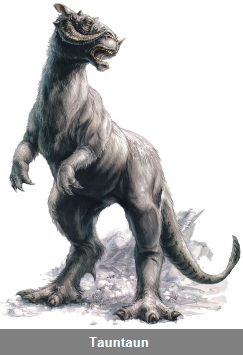
Figure 1.4: Figure retrieved on March 24, 2015 from http://starwars.wikia.com/wiki/Tauntaun.

In your duties as a biologist, you work with multiple datasets and are charged with analyzing data. You are further required to write an annual report summarizing population status, trends, and management activities. Because the public is interested in the Tauntaun population status, your report must be a sharp-looking PDF file and also an html file that can be housed on your organization’s website.

You will work with four datasets in your analysis:

Harvest dataset (a CSV file that contains information about Tauntauns that have been harvested)
Hunter dataset (a CSV file that contains hunter information, such as where the hunter lives)
Climate and weather datasets (CSV files obtained from NOAA)
Spatial datasets such as Vermont town boundaries (available from the Vermont Center for Geographic Information)

A CSV file is a file that stores data where each value is separated by commas; comma separated values. CSV files can be edited with Excel and read into R. R can also read Excel files directly.

In order to work with these datasets, you’ll use several functions that are included in the base R program, but you’ll also download additional “packages” that include functions that are not in the base R package. Some of the packages you’ll need are:

readxl - a package for reading from and writing to Excel spreadsheets
dplyr - a package for manipulating datasets
rmarkdown - a package for creating “markdown” documents, such as the one you are reading
rgdal - a package for reading spatial shapefiles
others.

Don’t worry about getting these packages right now….we’ll be retrieving and calling them when we need them throughout the primer exercises. And fear not, you will soon see (in Chapter 3) that installing packages is a very easy task.

1.4 Organization of the Primer

This primer is organized into chapters of varying length. The chapters are meant to be worked on in order:

You’re reading Chapter 1 now.
In Chapter 2 we’ll take a spin through RStudio.
In Chapter 3, we’ll learn more about functions and packages, and the concept of ‘libraries’. Everything that R does is done via a function.
Chapter 4’s focus is on “objects”, a critical concept in R. Everything that exists in R is an object.

Thus, Chapters 1 through 4 provide a basic introduction to R and RStudio. The remaining chapters center on your work as the Tauntaun biologist, where you will be introduced to several basic R techniques along the way.

Chapter 5 will discuss setting up a project in RStudio. You’ll learn how to create directories and inspect files in R, and how to download files from the web.
In Chapter 6 and 7, you’ll learn several commonly-used base R functions to clean up the data, a process known as “data wrangling”. These chapters introduce several commonly used base R functions.
Chapter 8 introduces the dplyr package for data wrangling.
Chapter 9 will focus on conducting basic statistical analysis, R’s bread and butter.
In Chapter 10, we’ll learn how to create a Tauntaun annual report with rmarkdown - this will be an automated reported that summarizes the number of animals harvested by town, county, age, sex, and harvest method; the report will be available as both a PDF file and an html file, viewable online and offline with any internet browser.
Chapter 11 will take the harvest analysis further . . . we’ll be developing a function (the sex-age-kill function) to estimate the living population size based on the harvested (dead) animals. This will give us an opportunity to learn some function building techniques and debugging methods.
In Chapter 12, we’ll create an R package so that you can send your custom sex-age-kill function to other Tauntaun biologists.
In Chapter 13 we spill the beans and show the if-then-else and looping methods that we used to simulate our Tauntaun datasets, mistakes and all.
Chapter 14 discusses various options for creating slideshows/presentations in R.

1.5 Assumptions

This primer is targeted at new users of R. We’ll assume that you have installed both R and R Studio.
We’ll assume that you know how to open R Studio and a bit about file directories (folders stored on your system) and how to navigate to them.
In order to install R packages, you’ll need to have internet access. R’s helpfiles and many R forums are accessed via the web as well.

Let’s get started.