Chapter 11 Writing Functions

Packages needed:
 * lubridate

11.1 Introduction

Aren’t you glad to have that pesky annual report out of the way? As the Tauntaun biologist, this report is just one of your many annual tasks – one that traditionally took 1 month to create. Hopefully your R markdown report will make this annual task a breeze. The report itself was simply a summary of the number of harvested animals sliced and diced in multiple ways, submitted to the Fish and Wildlife Service. But what do they do with the data you have reported? The answer: they do a population analysis.

As a trained wildlife biologist, you know that harvest data are just the beginning of a population analysis. As Gove et al. (2002) suggest, “Intriguingly nested within the age-at-harvest data is information on age and sex composition, survival, and fecundity rates.” In other words, our Tauntaun harvest data (which is full of records of dead animals of a particular age and sex) can be analyzed to estimate the size of the living Tauntaun population immediately before the harvest began. And if the population size is estimated each and every year, we can then look at trends in abundance through time, and think about what factors might affect this trend and how to manage it.

There are several methods for analyzing the age-at-harvest data, and here we will use two.

An index method. This method requires that user supplies the harvest rate and the harvest data, and the function will estimate the population size from these two inputs.
A simple method called the Sex-Age-Kill model. This model was developed by Lee Eberhardt in the 1960’s to estimate the population size of white-tailed deer. The original paper and worksheet outlining the method can be found on the Wisconsin Department of Natural Resources website.

Our goal is not a treatise on population estimation methods (nobody really uses the index method). Rather, we’ve selected this exercise as a means for teaching you how to create a function in R and how to loop through analyses using both looping methods and R’s set of “apply” functions. In the next chapter, we’ll show you how to put your two new function into an R package so that you can share your function with other Tauntaun biologists. Let’s get started.

Open a new script file, and save it as chapter11.R. Do this now! Use this file to follow along the R code in this chapter. Later in the exercise, we will create two new script called index.R and sak.R, which will store our actual function code.

11.2 Functions

As you’ve seen in chapter 3, functions are the heart and soul of R. Everything that R does is done via a function. Hundreds of functions are included in the R base packages, and other functions are contributed in the form of add-in packages.

Before going any further, let’s use a function, and then look at how it was coded. First, let’s load the package, lubridate.

# load the package, lubridate
library(lubridate)

Remember that when you load a package, you can find it in the Environment tab by clicking on the small drop-down arrow next to the word Global Environment

Click on the lubridate option, and you should see the following.

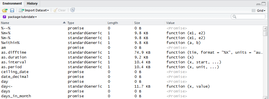
Figure 11.1: New R Markdown file.

What you are looking at are the functions that come with the lubridate package. Look for the function called days_in_month. Now, let’s see what the days_in_month function does.

help(days_in_month)

This function has just one argument, x, in which a user passes in a datetime object. Let’s try it:

# determine number of days in February in 1901
days_in_month(as.Date("1901-02-01"))

## Feb 
##  28

# determine number of days in February in 1980, a leap year
days_in_month(as.Date("1980-02-15"))

## Feb 
##  29

This seems like a pretty straight-forward and useful function.

One very nice thing about R is that you can actually see the function code by just typing in the function name (with no parentheses or arguments):

# look at the code for the function, days_in_month
days_in_month

## function (x) 
## {
##     month_x <- month(x, label = TRUE, locale = "C")
##     n_days <- N_DAYS_IN_MONTHS[month_x]
##     n_days[month_x == "Feb" & leap_year(x)] <- 29L
##     n_days
## }
## <bytecode: 0x000000001f61c6e8>
## <environment: namespace:lubridate>

Here, we can see the code for the days_in_month function, written by the lubridate package authors. This function “lives” in an environment that has a name of lubridate. Let’s use the packageDescription function to learn more about the package:

packageDescription(pkg = 'lubridate')

## Type: Package
## Package: lubridate
## Title: Make Dealing with Dates a Little Easier
## Version: 1.7.9
## Authors@R: c(person(given = "Vitalie", family = "Spinu", role = c("aut", "cre"), email = "spinuvit@gmail.com"), person(given =
##                "Garrett", family = "Grolemund", role = "aut"), person(given = "Hadley", family = "Wickham", role = "aut"),
##                person(given = "Ian", family = "Lyttle", role = "ctb"), person(given = "Imanuel", family = "Costigan", role = "ctb"),
##                person(given = "Jason", family = "Law", role = "ctb"), person(given = "Doug", family = "Mitarotonda", role = "ctb"),
##                person(given = "Joseph", family = "Larmarange", role = "ctb"), person(given = "Jonathan", family = "Boiser", role =
##                "ctb"), person(given = "Chel Hee", family = "Lee", role = "ctb"))
## Maintainer: Vitalie Spinu <spinuvit@gmail.com>
## Description: Functions to work with date-times and time-spans: fast and user friendly parsing of date-time data, extraction and
##                updating of components of a date-time (years, months, days, hours, minutes, and seconds), algebraic manipulation on
##                date-time and time-span objects. The 'lubridate' package has a consistent and memorable syntax that makes working with
##                dates easy and fun.  Parts of the 'CCTZ' source code, released under the Apache 2.0 License, are included in this
##                package. See <https://github.com/google/cctz> for more details.
## License: GPL (>= 2)
## URL: http://lubridate.tidyverse.org, https://github.com/tidyverse/lubridate
## BugReports: https://github.com/tidyverse/lubridate/issues
## Depends: methods, R (>= 3.2)
## Imports: generics, Rcpp (>= 0.12.13)
## Suggests: covr, knitr, testthat (>= 2.1.0), vctrs (>= 0.3.0)
## Enhances: chron, timeDate, tis, zoo
## LinkingTo: Rcpp
## VignetteBuilder: knitr
## Encoding: UTF-8
## LazyData: true
## RoxygenNote: 7.1.0
## SystemRequirements: A system with zoneinfo data (e.g. /usr/share/zoneinfo) as well as a recent-enough C++11 compiler (such as g++-4.8
##                or later). On Windows the zoneinfo included with R is used.
## Collate: 'Dates.r' 'POSIXt.r' 'RcppExports.R' 'util.r' 'parse.r' 'timespans.r' 'intervals.r' 'difftimes.r' 'durations.r' 'periods.r'
##                .....
## NeedsCompilation: yes
## Packaged: 2020-06-03 11:12:59 UTC; vspinu
## Author: Vitalie Spinu [aut, cre], Garrett Grolemund [aut], Hadley Wickham [aut], Ian Lyttle [ctb], Imanuel Costigan [ctb], Jason Law
##                [ctb], Doug Mitarotonda [ctb], Joseph Larmarange [ctb], Jonathan Boiser [ctb], Chel Hee Lee [ctb]
## Repository: CRAN
## Date/Publication: 2020-06-08 15:40:02 UTC
## Built: R 4.0.2; x86_64-w64-mingw32; 2020-07-16 21:02:47 UTC; windows
## 
## -- File: C:/RSiteLibrary/lubridate/Meta/package.rds

There are quite a few contributors to this package; now we know who to thank.

We’ll run through their code in a minute, but for now we’re interested in understanding the structure of a function, which is very specific and along the lines of:

my.function  <- function(arg1, arg2, ... ){

  the function's code (body) is nestled between curly braces
  
  return(object)
  
}

To create a function, we start by assigning the function a name with the assignment operator, such as my.function <-. This names the function; if the name is omitted, the function is called an anonymous function (functions without names). To save a function, it must be named.

Then, we use the function function (you read that correctly!) to tell R it will be a function. We list the arguments in our function between parentheses and include any default values. These are the function’s inputs. Then, in between two curly braces { }, we enter R code that tells R what to do with the inputs, and what to return to the function user (the output).

Can you see these elements in the days_in_month function?

function (x) 
{
    month_x <- month(x, label = TRUE, locale = "C")
    n_days <- N_DAYS_IN_MONTHS[month_x]
    n_days[month_x == "Feb" & leap_year(x)] <- 29L
    n_days
}

There is just one argument, called x. We already know that a user will input a datetime object. In between the curly braces are the instructions, or function body. Let’s look at them line-by-line:

The authors first use the month function (which is also a function in lubridate) to extract the month from the input datetime object. This result is stored as a new object called month_x:
- month_x <- month(x, label = TRUE). This function will return something like this: “Feb” (which is an ordered factor level).
They then create a vector called n_days, which provides the number of months for each day of the year. This is done with the N_DAYS_IN_MONTHS function, passing in month_x as the argument. This will return the value 28.
Next, if the month_x is February and if the original input date it is a leap year (identified with another lubridate function called leap_year), the element in n_days changes to 29:
- n_days[month_x == “Feb” & leap_year(x)] <- 29L. Here, the “L” indicates that 29 is an integer.
Finally, the object n_days is returned to the global environment:
- n_days. This could have been written return(n_days), but R will always return the last object if omitted.

Seems pretty straight-forward, doesn’t it? Notice that the sequence of commands within the function is important, with each line building on objects created in previous lines. Let’s run their code and see first-hand what each line is doing. Here, we wrap each line of code in parentheses so that R executes the code and returns the result.

# enter Nelson Mandela's birthday as a date object called x
(x  <- as.Date("1918-07-18"))

## [1] "1918-07-18"

# retrieve the month of Mandela's birthday with the month function
(month_x <- month(x, label = TRUE))

## [1] Jul
## Levels: Jan < Feb < Mar < Apr < May < Jun < Jul < Aug < Sep < Oct < Nov < Dec

# set up a named vector of day
(n_days <- 31L)

## [1] 31

# if month_x is Feb and x is a leap year, replace the days with 29.
(n_days[month_x == "Feb" & leap_year(x)] <- 29L)

## [1] 29

# return the object n_days
n_days

## [1] 31

The number 31 is returned for Nelson Mandela’s birthday because July has 31 days. One line may have tripped you up here, and that is the code that forces July to have 31 days (n_days <- 31L). We did that because the function N_DAYS_IN_MONTHS is not available for users (it is an “internal” function).

Why would the authors write this function? Well, the chief reason to create a custom function is to avoid re-coding the same set of instructions over and over again. In the case of lubridate, the authors combine a whole suite of functions to make it easier to work with dates and times, things that almost all R users will encounter at some point or another. (Thank you!)

The function function allows the creation of a function. Let’s take a look at this function in the helpfile, noting that the word “function” must be quoted to locate the help page.

help("function")

Read this helpfile now. The arguments of the function function are the arglist (which is a list of function’s arguments enclosed within a set of parentheses, each separated by commas), expr (an expression or set of code that tells R what calculations to perform, which is nestled between curly braces), and value (which signifies what to return). Be aware that although these are the arguments to the function function, you won’t actually include these argument names when you build a function.

As the Tauntaun biologist, you need to estimate the population size of the Tauntauns each and every year based on the Tauntaun harvest. You certainly don’t want to write the code for one year, and then re-write it for a second year.

Any time you you use code repeatedly to do a task, you should think of making it into a function.

Let’s start by making a very simple function, and then move to our harvest functions.

11.3 Your First Function

As a first attempt, let’s create a function that squares a number that is input into the function. Are you ready? Let’s call our function sq.function.

ADD BOX DIAGRAM HERE

Copy the following code into script now, and run it:

sq.function  <- function(x){
  result  <- x^2
  return(result)
  }

This function has one input named x, which the user of the function will supply. That makes up our short but sweet argument list (arglist). Inside the curly braces, we tell R to square x (which the user supplied) and store the answer in a new object called result. This makes up our expression (expr argument). Then we use the return function to have R return the result. The object called result makes up our return argument. The expression and value are enclosed within curly braces.

You need to execute this code (i.e., source it) for R to use it.

After you’ve run this code, look for it in your Global Environment.

Your function is another object in R, and you should see that its type is function. Our function is a real, user-supplied extension of R’s capabilities. We haven’t written a manual page, nor have we made it into a package, but we can query its arguments, check its class, and return the source code:

# get the class for the sq.function
class(sq.function)

## [1] "function"

# get the arguments for the sq.function
args(sq.function)

## function (x) 
## NULL

# now view the code for the sq.function
sq.function

## function(x){
##   result  <- x^2
##   return(result)
##   }

All seems to be in order. Let’s test our new function by squaring the number 3:

# use the function sq.function
sq.function(3)

## [1] 9

Not bad! This is a pretty straight-forward function. When you entered the number three between parentheses, you passed that value to the function – the value is now stored in R’s “function environment” (not the global environment), where is it used in the function’s body. More on this topic later . . .

Let’s try it again, this time storing our answer as a new object:

# use the function sq.function; store the result
my.answer <- sq.function(3)

# show the result
my.answer

## [1] 9

In writing functions, just as in writing a paper, you must pay attention to the function user. Consider these ditties:

“Essentially style resembles good manners. It comes of endeavouring to understand others, of thinking for them rather than for yourself – or thinking, that is, with the heart as well as the head.” – Sir Aurthur Quiller-Couch

“And how is clarity to be achieved? Mainly by taking trouble; and by writing to serve people rather than to impress them.” – F. L. Lucas

In other words, it’s a good idea to think of how a user will use your function, the various ways in which the function can throw errors, and hints or tips that might help put your user on the right track.

Suppose, for example, the user supplies a character element to your function:

sq.function("three")

Here, R generates an error:

Error in x^2 : non-numeric argument to binary operator

This says that x is a numeric argument, but we passed a value to it that is non-numeric, and R can’t carry out the operation. If you think your user will not be able to decipher this message easily, you may consider adding message, warning and/or stop functions within your function to give the user some feedback. These are intended to limit misuse of your function. We’ll use these shortly. If you will be the only user of your function, of course you may take more liberties.

Here, though, we’ll assume that you are writing your two harvest analysis functions not only for yourself, but for some of your colleagues in other states who also work on Tauntauns. That means you’ll need to put your user first when writing code. However, since you’ll be the main user, we’ll want to make the function easily work with our Tauntaun dataset.

Let’s read in our super-cleaned and merged TauntaunData.RDS file and remind ourselves how it is structured:

# read in the Tauntaun dataset
TauntaunHarvest <- readRDS("datasets/TauntaunData.RDS")

# look at its structure
str(TauntaunHarvest)

## 'data.frame':	13352 obs. of  19 variables:
##  $ hunter.id    : num  560 89 49 108 225 633 146 12 602 462 ...
##  $ age          : num  1 1 3 3 1 3 1 1 1 4 ...
##  $ sex          : Factor w/ 2 levels "f","m": 1 1 2 1 2 1 2 1 2 2 ...
##  $ individual   : num  116 53 822 795 468 809 347 144 384 902 ...
##  $ species      : chr  "Tauntaun" "Tauntaun" "Tauntaun" "Tauntaun" ...
##  $ date         : Date, format: "1901-10-01" "1901-10-01" "1901-10-01" "1901-10-01" ...
##  $ town         : Factor w/ 255 levels "ADDISON","ALBANY",..: 1 21 90 93 96 134 146 158 224 8 ...
##  $ length       : num  294 315 427 270 448 ...
##  $ weight       : num  677 880 1039 624 1109 ...
##  $ method       : Factor w/ 3 levels "bow","lightsaber",..: 2 1 3 2 2 1 3 2 2 2 ...
##  $ color        : Factor w/ 2 levels "White","Gray": 1 2 1 2 1 2 2 2 2 2 ...
##  $ fur          : Factor w/ 3 levels "Short","Medium",..: 3 3 2 2 3 1 3 1 2 3 ...
##  $ month        : num  10 10 10 10 10 10 10 10 10 10 ...
##  $ year         : num  1901 1901 1901 1901 1901 ...
##  $ julian       : num  274 274 274 274 274 274 274 274 274 275 ...
##  $ day.of.season: num  1 1 1 1 1 1 1 1 1 2 ...
##  $ sex.hunter   : Factor w/ 2 levels "f","m": 2 2 2 2 2 1 2 2 2 2 ...
##  $ resident     : logi  FALSE TRUE TRUE TRUE TRUE TRUE ...
##  $ count        : num  1 1 1 1 1 1 1 1 1 1 ...

Our goal now is to create two new functions, index and sak, that will estimate the size of the living Tauntaun population based on the harvest records.

11.4 Steps to Writing a Function

Before we go too far, let’s think about our function-creating process. The steps to writing a custom function are:

Identify the necessary inputs and determine how the user will provide them.
Identify the desired outputs (and how they will be used).
Develop a ‘word’ prototype of the function; this means write out the steps in words. At this stage, don’t worry about R coding . . . we are concerned with the logical flow of steps. A box diagram would be helpful here too.
Add the R the calculations to the correct spot.
Debug the function.

11.5 The Index Function

Our first function will be called the index function.

Open a new script, and name it index.R. This script will contain the index function code; we will be able to use this script in our next chapter.

Here’s the rationale behind our homemade index function. If you know the total population size of Tauntauns (called N), and you know the harvest rate, (called r), then you can easily compute the total number of individuals that you expect to be harvested (called H) .

\[ N * r = H\]

For example, if the Tauntaun population size is 100, and the harvest rate is 0.2, then we expect 20 Tauntauns will be harvested.

Now, if we have 20 harvested Tauntauns, and we know what r is, we can estimate N as:

\[N = \frac{H}{r} = \frac{20}{0.2} = 100\] So, our function requires that the user will input annual harvest data (which will give us $H$), and will input the harvest rate (which will give us $r$). The function can then do this calculation and return the output. We can start a bare-bones function like this:

index <- function(annual_harvest, 
                  prob_of_harvest) {
  
  
} # end of function

Run this code, then look for this function in your Global environment. This function doesn’t do anything yet: there is nothing in the function’s body. But, we have defined our two arguments (annual.harvest and prob_of_harvest), so that’s a start.

Do we need more arguments than that? While the user might enter something like 0.2 for the prob_of_harvest argument, what exactly do we want the user to pass in for annual_harvest? For example, do you want the user to pass in a dataframe? If so, how should this dataframe be structured? Or do we want the user to pass in just the total number of harvested animals, in which case the user would need to calculate this number before using the index function. These are the questions you must ponder before you start writing the function body.

Our Tauntaun harvest dataset has many years of data, and we don’t want to have to take the time futzing with it to trim it by year. Let’s suppose we decide that our index user will pass in the entire harvest dataset, and have the function do the subsetting. In this case, we need to adjust our arguments: harvest_data will be the full Tauntaun dataset, year will be the year of interest, and prob_of_harvest will be the probability of harvest. Of course, we’ve made some big assumptions here about what the harvest dataset will look like. We’ll assume that the data are structured as a dataframe with a column named “year”. Further, we will assume that each row in the dataset represents a single harvested Tauntaun (as our dataset is currently formatted). With this in mind, let’s start again!

index <- function(harvest_data, 
                  year,
                  prob_of_harvest) {
  
  
} # end of function

Our function still doesn’t do anything yet because there is nothing in the function’s body. Let’s add in some comments to our function’s body now to help us track the operational steps. Assuming the users passes in a dataframe of harvest data, our code can first test if the column named “year” is present in the harvest dataset. Next, we can subset the dataset by year. Then, we can sum the total harvest. Then, using the prob_of_harvest argument, we can calculate the result, and then return it to the user. Let’s add notes as comments in the function body:

index <- function(harvest_data, 
                  year,
                  prob_of_harvest) {
  
  # test if the dataset has a column named "year"
  
  # subset the data by year
  
  # sum the harvest
  
  # calculate the result
  
  # return the result
  
} # end of function

Next, let’s add code under each comment. Here, we’ll be using functions that we have encountered in previous chapters, so we won’t spend too much time discussing their nuances:

index <- function(harvest_data, 
                  year,
                  prob_of_harvest) {
  
  # test if the dataset has a column named "year"
  if ("year" %in% names(harvest_data) == FALSE) stop("Your harvest dataset must have a column
                                                     named 'year'.  Further, each row in your
                                                     dataset is assumed to represent 1
                                                     Tauntaun.")
  
  # subset the data by year
  indices <- which(harvest_data$year == year)
  annual_harvest <- harvest_data[indices, ]
  
  # sum the harvest
  total_harvest <- nrow(annual_harvest)
  
  # calculate the result
  estimate <- total_harvest/prob_of_harvest
  
  # return the result
  return(estimate)
  
} # end of function

There you have it, our index function. Most of this code is straight-forward. The only new element that may need some explanation is the if-stop syntax. First, we ask if the word “year” is in the names of the harvest_data with the %in% operator. If this result is FALSE, the stop function is executed, which breaks the function and returns a message to the user: “Your harvest dataset must have a column named ‘year’.”

While we mapped out out our function first in words, some people like to map out their functions as flow charts.

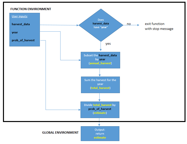
Flowchart courtesy of Jacob Weissgold. The inputs (black) become part of the function's environment. New objects (yellow) are created in the function environment. The final output is returned to the Global Environment.

Figure 11.2: Flowchart courtesy of Jacob Weissgold. The inputs (black) become part of the function’s environment. New objects (yellow) are created in the function environment. The final output is returned to the Global Environment.

The code produces an object called estimate (which is our population estimate), and this object is returned to the user with the return function.

Now, click on the box that says “Source on Save”, and then save your script. This will source your function any time your script is saved. Alternatively, press the “Source” button, which will source the script on command. “Source” means “send your function to R’s global environment, ready to be used.” Our function “lives” in the global environment, unlike the days_in_month function, which lives in the lubridate environment, or the readOGR function, which lives in the rgdal environment. You can also source your function by clicking on the Source button in the upper right corner of the script editor. Make sure you look for your index function in the global environment!

11.5.1 Testing the index function

Let’s test our function for the year 1901 in your console (don’t add this to your function!):

index(harvest_data = TauntaunHarvest, 
                  year = 1901,
                  prob_of_harvest = 0.2)

## [1] 4655

Let’s test our function for the year 1910 in your console:

index(harvest_data = TauntaunHarvest, 
                  year = 1910,
                  prob_of_harvest = 0.2)

## [1] 8370

It works! At least we think it works at this point. We could add much more to this function if we wished. For instance, we could check to make sure that the probability of harvest is between 0 and 1. Additionally, we could have included confidence in our estimate by invoking the binomial distribution to compute our estimate instead of simple division. But we’ll keep this function short and sweet, as our goal here is talk about functions in R and not population analysis.

11.6 The Sex-Age-Kill Function

Our second function is called the sex-age-kill function. Unlike the index function, this function is actually used by many state agencies to estimate the population size of animals just before the harvest. The original paper and worksheet outlining the method can be found on the Wisconsin Department of Natural Resources website.

In the preface, the author notes “This report is a compromise, and like all compromises, will probably be unsatisfactory from several points of view. The biologist may find too much mathematics here, but the biometrician or statistician will quite surely find the analysis to be inadequate and incomplete in several respects. Those responsible for field management of deer herds will very likely find too many of the results given here to be either contradictory or not sufficiently explicit for direct application.” That’s quite a disclaimer! We will simply follow the steps and not worry too much about these details. Again, our aim in this chapter is to focus on the mechanics of writing a function.

Open a new R script, and save it as sak.R.

Let’s quickly overview what the SAK estimator does. The approach estimates the total, pre-harvest population size for a given year, and requires that each animal is identified into one of four age groups:

Young = 0-year-olds.
Juveniles = individuals > 0 but not yet of breeding age (juveniles).
Recruits = individuals in their first year of breeding. They are called recruits because they have been recruited into the breeding population.
Adults = individuals who have had at least one year of breeding under their belt.

It is well known that Tauntauns breed at age 1, and harvest begins at that age as well. So the harvest dataset should consist only of recruits (first year breeders) and adults (experienced breeders). Because recruit and adult age groups consist of breeding individuals, we will use the word “breeders” to represent the total breeding population. (Incidentally, the names of these age groups were not originally used by Eberhardt, who used deer-related terms).

Although the SAK approach involves several calculation steps, all of them are simple (involving addition, multiplication, and division). As with our index function, the user will need to supply a harvest dataset and the year of interest. Further, the user will need to provide two more inputs to the function. First, they will provide an estimate of the percentage of the annual mortality is due to harvest. For example, if we think that 90% of the total adult male mortality is due to harvest, we would enter 0.9 for this input. This means that 10% of the total mortality is due to natural causes. Second, the user will provide an estimate of the female per capita birth rate.

So our function inputs will be:

harvest_data = the data frame containing the harvest data
year = the year of the analysis
proportion_mortality_harvest = the proportion of the total annual adult mortality for males that is due to harvest
offspring_per_female = the average number of offspring per adult female.

Remember, as the function developer, you can choose any name you want for your arguments, but clarity is the name of the game. The developer of the days_in_month function named his or her argument x, but they could have also named it input_date if they wanted. The names of our sak arguments are a bit long-winded, but we’ll use these long names so you don’t have to wonder they mean.

To use this function, we will make the bold assumption that the harvest_data will be contain columns named “age”, “sex”, and “year” (as occurs in our Tauntaun data), and that each row in the dataset represents a single Tauntaun. Furthermore, we will assume that ages are listed as integers (e.g., 0, 1, 2, 3, . . . ) and that sexes are identified as “m” and “f”.

We have enough information now to start our sak function. This is our starting point:

sak <- function(harvest_data, year, proportion_mortality_harvest, offspring_per_female = 2){
  
  # the function body will go here
  
} # end of function

Notice that only one of our arguments has a default value. Can you find it? Yup . . . the argument offspring_per_female has a default value of 2. To add a default value, simply add an equal sign and value after the argument name (e.g., offspring_per_female = 2). The writer of the function chooses any default values, which is why you should always, always double-check default values for every function you use!

What should go in the function body? The key calculations are shown below:

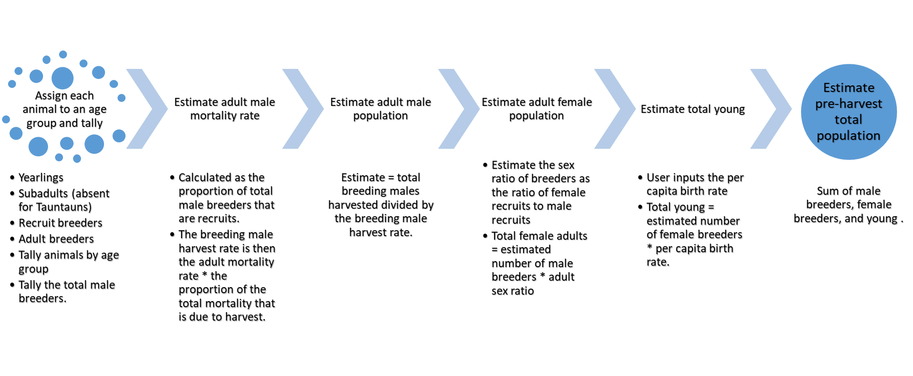
Figure 11.3: The sex-age-kill calculations.

Next, we’ll add the key steps as comments to our function, and the fill in the R code later. You may think it is a pain to write out the thought-process in words, but this process helps you link the inputs with the outputs. As a side note, don’t worry too much about the actual calculations . . . we’ll provide the calculations for you so you don’t have to remember each step. Our goal is to have you develop a function - not to become an expert in the nuances of the SAK estimator. Here we go:

sak <- function(harvest_data, year, proportion_mortality_harvest, offspring_per_female = 2){
  
  # ensure the columns "age", "sex", and "year" are present in the harvest_data
  
  # ensure the proportion_mortality_harvest is between 0 and 1
  
  # subset the data by year
  
  # assign each animal to an age group
  
  # tally the individuals by age group
  
  # tally the total male breeders
  
  # estimate adult male annual mortality as the proportion of total breeding males that are recruits
  
  # estimate the breeding male harvest rate as the mortality rate * proportion_mortality_harvest
  
  # estimate the total living breeding male population size as breeding male harvest / harvest rate
  
  # estimate the sex ratio as the ratio of female recruits to male recruits
  
  # estimate the total breeding female population size as the breeding male pop * sex ratio
  
  # estimate the total offspring produced as the breeding female pop * offspring_per_female
  
  # estimate the pre-harvest population size as the sum of male breeders, female breeders, and young 
  
  # create the results as a list  
  
  # return the results
  
} # end of function

The last part of any function is the object to be returned, and only one object can be returned. Let’s think about this. The main output for our function will be an estimate of population size. But we could include other outputs as well. Let’s identify a few of them:

pop.est = the estimate of the total population size (pre-harvest)
harvest.rate = the harvest rate of adult males
breeding.male.est = the estimate of the breeding male population size
breeding.female. = the estimate of the breeding female population size
offspring.est = the estimate of the offspring population

Given this, it makes sense that we return the result as a list. To begin our function, type (or copy) in the following into “sak.R”. We will talk about the code itself later.

sak <- function(harvest_data, year, proportion_mortality_harvest, offspring_per_female = 2){
  
  # ensure the columns "age", "sex", and "year" are present in the harvest_data
  if (all(c("age", "sex", "year") %in% names(harvest_data)) == FALSE) stop(
    "Your harvest dataset must contain columns named 'year', 'age', and 'sex'.  
    Further, each row in the dataset must represent a single Tauntaun.")
  
  # ensure the proportion_mortality_harvest is between 0 and 1
  if (any(proportion_mortality_harvest <= 0, proportion_mortality_harvest > 1)) stop(
    "The input, prop_mortality_harvest must be between 0 and 1.")
  
  # subset the data by year
  indices <- which(harvest_data$year == year)
  annual_harvest <- harvest_data[indices, ]
  
  # assign each animal to an age group
  annual_harvest$agegroup <- ifelse(annual_harvest$age == 1, yes = "recruit", no = "adult")

  # tally the individuals by age group
  harvest_freq <- table(annual_harvest$agegroup, annual_harvest$sex)
  
  # tally the total male breeders
  total_breeding_males  <- sum(harvest_freq[,'m'])
  
  # estimate adult male annual mortality as the proportion of total breeding males that are recruits
  annual_mortality_rate  <- harvest_freq['recruit', 'm']/total_breeding_males
  
  # estimate the breeding male harvest rate as the mortality rate * proportion_mortality_harvest
  harvest_rate  <- annual_mortality_rate * proportion_mortality_harvest
  
  # estimate the total living breeding male population size as breeding male harvest / harvest rate
   breeding.male.est  <- total_breeding_males / harvest_rate
   
  # estimate the sex ratio as the ratio of female recruits to male recruits
   sex_ratio  <- harvest_freq['recruit', 'f']/harvest_freq['recruit', 'm']
  
  # estimate the total breeding female population size as the breeding male pop * sex ratio
   breeding.female.est  <- breeding.male.est  * sex_ratio
  
  # estimate the total offspring produced as the breeding female pop * offspring_per_female
   offspring_est  <- breeding.female.est * offspring_per_female
  
  # estimate the pre-harvest population size as the sum of male breeders, female breeders, and young
  pop_est  <- round(breeding.male.est + breeding.female.est + offspring_est, digits = 2)
  
  # create the results as a list 
  results  <- list('Total Population Estimate' = pop_est,
                     'Harvest Rate' = harvest_rate, 
                     'Total Male Adult Estimate' = breeding.male.est, 
                     'Total Female Adult Estimate' = breeding.female.est, 
                     'Total Offspring Estimate' = offspring_est)
    
  # return the results
  return(results)
  
} # end of function

Take care to keep your code sharp-looking in terms of spacing, commenting, and indenting. These will not affect the way the code is executed, but they certainly affect the sanity of the coder!

That’s a long(ish) function. Can you imagine typing this code each time you want to run the SAK estimator? By storing the code as a function, and letting the user specify unique inputs, you can simply call up the function and use it at will.

Writing functions is not for just elite coders . . . in R, you can create functions to automate any tasks that you repeatedly do.

Let’s run through the function body code step by step. These can be run in the console, or in a new script called chapter11.R if you wish. Don’t add this code to your function! First, let’s assume we provide the following inputs to the function

TauntaunHarvest <- readRDS("datasets/TauntaunData.RDS")
harvest_data <- TauntaunHarvest
year <- 1901
proportion_mortality_harvest <- 0.5
offspring_per_female <-  2

Next, we need to ensure that the harvest dataset includes the column names of “age”, “sex”, and “year”. The function won’t work without knowing this information. Here, we ask if these names are in the column names of the harvest data, again using the %in% operator. This will return a vector of 3 TRUE values if they are all present. The function all is a quick way to ask if all of the elements are TRUE. If this evaluates to FALSE, then one of our columns is missing, and the function will stop and send the user an error message:

# ensure the columns "age", "sex", and "year" are present in the harvest_data
if (all(c("age", "sex", "year") %in% names(harvest_data)) == FALSE) stop(
    "Your harvest dataset must contain columns named 'year', 'age', and 'sex'.  
    Further, each row in the dataset must represent a single Tauntaun.")

Next, we’ll make sure that the user has entered a proportion (a number between 0 and 1), and will force the function to “stop” if these conditions are not met. The code any(proportion_mortality_harvest <= 0, proportion_mortality_harvest > 1) will evaluate two conditions, and ask if any of these are TRUE. If either is TRUE, we have an invalid input, and the function will stop and return a message to the user:

# ensure the proportion_mortality_harvest is between 0 and 1
if (any(proportion_mortality_harvest <= 0, proportion_mortality_harvest > 1) == TRUE) stop(
    "The input, proportion_mortality_harvest must be between 0 and 1.")

Next we subset the harvest data by the year of interest. Here, we determine which rows match our year condition, and store those row numbers in a vector called indices. Then we use bracket subsetting to subset the data:

# subset the data by year
indices <- which(harvest_data$year == year)
annual_harvest <- harvest_data[indices, ]

At this point, we have an annual dataset. Our next step is to add a column called agegroup. Here, we will use an ifelse function to return an agegroup of “recruit” for Tauntauns of age 1, and “adult” for Tauntauns of any other age. Remember, Tauntaun harvest begins at age 1, and these are also our first-year breeders (recruits). Our dataset will thus include only individuals of age group “recruit” or “adult” (collectively known as “breeders”).

# assign each animal to an age group
annual_harvest$agegroup <- ifelse(annual_harvest$age == 1, yes = "recruit", no = "adult")

Our next step will be to count the total harvest by sex by age group. A quick way to do this is to use the table function.

# tally the individuals by age group
harvest_freq <- table(annual_harvest$agegroup, annual_harvest$sex)

Now we’re rolling. Next, we tally **all* breeding males (recruits and adults = breeding males).

# tally the total male breeders
total_breeding_males  <- sum(harvest_freq[,'m'])

Next, we estimate the total male mortality rate as the percentage of breeders that are recruits. Why this is an estimate of adult male mortality rate is explained by Eberhardt.

# estimate breeding male annual mortality as the proportion of total breeding males that are recruits
annual_mortality_rate  <- harvest_freq['recruit', 'm']/total_breeding_males

This is the total mortality rate of breeding males, which can be decomposed into mortality due to harvest (harvest_rate) and mortality due to natural causes. We can estimate the adult male harvest rate (harvest_rate) as the annual_mortality_rate times the proportion of total mortality due to harvest (proportion_mortality_harvest), which if you recall has been provided by the user.

# estimate the breeding male harvest rate as the mortality rate * proportion_mortality_harvest
harvest_rate  <- annual_mortality_rate * proportion_mortality_harvest

At last we are ready for our first estimate, which will be the total male breeder population (recruits and adult breeders). This will simply be a count of the total male adult harvest divided by the harvest rate.

# estimate the total living breeding male population size as breeding male harvest / harvest rate
breeding_male_est  <- total_breeding_males / harvest_rate

Now that we have an adult male population estimate, it’s time to estimate the adult female population size. To do so, we need an estimate the sex ratio of adult females/adult males. For Tauntauns, the best estimate of adult sex ratio is to consider the sex ratio of only recruit adults, which we do here:

# estimate the sex ratio as the ratio of female recruits to male recruits
sex_ratio  <- harvest_freq['recruit', 'f']/harvest_freq['recruit', 'm']

Now that we have a sex ratio estimate of adults, we can estimate the total female population size by multiplying the total estimated male population by the sex ratio:

# estimate the total breeding female population size as the breeding male pop * sex ratio
breeding_female_est  <- breeding_male_est  * sex_ratio

Almost there! Now that we have an estimate of the breeding female population size, we can estimate the total number of young as breeding.female.est times the per capita birth rate, which our user may have provided in the argument, offspring_per_female (if not, the default value of 2 is used).

# estimate the total offspring produced as the breeding female pop * offspring_per_female
offspring_est  <- breeding_female_est * offspring_per_female

And now for the grand finale, we can compute the total population size as the sum of the adults and offspring. Notice that this computation does not include juveniles. Since Tauntauns breed at age 1, there will be no juveniles in our population. But if another user applied this model to a species that, say, breeds at age 3, then the function would need some modification to account for these individuals. So, as it stands, our function assumes that individuals breed at age 1. As with any analysis, the result is interpreted bearing in mind the many biological assumptions of SAK and the spatial extent of our data.

# estimate the pre-harvest population size as the sum of male breeders, female breeders, and young 
pop_est  <- round(breeding_male_est + breeding_female_est + offspring_est, digits = 2)

To this point, we have created several objects within our function environment. Now we need to think about what object to return to the user. Previously, we indicated that we would like to return:

pop_est = the estimate of the total population size (pre-harvest)
harvest_rate = the harvest rate of adult males
breeding_male_est = the estimate of the breeding male population size
breeding_female_est = the estimate of the breeding female population size
offspring_est = the estimate of the offspring population

Since we can only return one object, we can stuff these objects into a list, and then return the list.

# create the results as a list 
results  <- list('Total Population Estimate' = pop_est,
                 'Harvest Rate' = harvest_rate, 
                 'Total Male Adult Estimate' = breeding_male_est, 
                 'Total Female Adult Estimate' = breeding_female_est, 
                 'Total Offspring Estimate' = offspring_est)

11.6.1 Testing the sak function

To test the function, we must send the function to R (i.e., source it) so that the function becomes an object within the global environment. You can source the function by pressing the source button or by selecting Code | Source. These actions invoke the source function, which “causes R to accept its input” (in our case, the function).

If your code has any errors in it, you’ll get an error message from R after attempting to source the function. These errors would be syntax errors . . . errors in coding such as not closing a parenthesis, spelling an object’s name incorrectly, etc. etc. As long as your code is free of such errors, the source function will run and you’ll see the function appear in your global environment. Note: this doesn’t mean that the code is 100% error free . . . more on this in a bit. If you change any of the code in your function, you must source it again in order for R to use the most current version. In RStudio, the Source on Save option conveniently sources your function whenever you save it Make sure this option is checked. Click on the Source on Save button, and then save your sak.R file now! The function should now appear in your Global Environment.

Now let’s give the SAK function a whirl.

Let’s assume we are interested in estimating the 1901 Tauntaun population size (pre-harvest, that is). Let’s enter 0.5 for proportion_mortality_harvest, and use the default birth rate:

# run the SAK function with appropriate arguments
results <- sak(harvest_data = TauntaunHarvest,
    year = 1901,
    proportion_mortality_harvest = 0.5,
    offspring_per_female = 2)

# show the results
results

## $`Total Population Estimate`
## [1] 6242.6
## 
## $`Harvest Rate`
## [1] 0.3061224
## 
## $`Total Male Adult Estimate`
## [1] 1440.6
## 
## $`Total Female Adult Estimate`
## [1] 1600.667
## 
## $`Total Offspring Estimate`
## [1] 3201.333

It worked! According to this estimator, the Tauntaun population estimate for 1901 is 6242.6 animals.

Many R functions will deliver output in the form of a list. Remember that a list is like a shoestore . . . it can holds objects of all types. To see what’s inside the list, use the trusty str function, and to pull shoeboxes out of this shoestore, use one of the extractor functions $ or [[ ]].

str(results)

## List of 5
##  $ Total Population Estimate  : num 6243
##  $ Harvest Rate               : num 0.306
##  $ Total Male Adult Estimate  : num 1441
##  $ Total Female Adult Estimate: num 1601
##  $ Total Offspring Estimate   : num 3201

We mentioned that just because the SAK function was successfully sourced, that does not mean it is error free. Coding errors come in a variety of flavors, and bad R syntax is the “best” sort of error to make. Why? Because R won’t run and will quickly let you know there is a problem. Other kinds of errors, though, are much more deceptive, and these include semantic errors and logic errors. For example, suppose that the harvest rate estimate was mistakenly coded as annual_mortality_rate / proportion_mortality_harvest. The code may very well run, but the output will be incorrect. This is a logic error; the code is correct but there is a logical mistake in your coding. In other words, it’s not sufficient to simply source the function . . . you must carefully check it and debug it as well.

11.7 Thoughts on Coding Style

We now have two functions, and this is a good time to quickly chat about coding styles for writing functions. Our functions are pretty short, but you can imagine that functions can get super long and complex. When that happens, consider breaking your functions into sets of smaller functions. See the chapter on Functions in R for Data Science for more information.

11.8 Debugging

Broken code is frustrating, but with a systematic strategy, errors can be identified and rectified quickly. The process of locating errors in code is known as debugging.

There are two ways to debug your code. You can enter the inputs that the function needs (as objects), and then run through the function’s body (the portion between the curly braces) line-by-line, clicking the ‘run’ button in RStudio or pressing Ctrl+return to send each line to the console. We sort of did this when stepping through the sak function. If you are running your script line-by-line, you will notice an error in your console when a command evaluates to an error. The root of the error may be in that line, or it may be in an input to a function or expression in that line. Either way, the cause of the error can be narrowed down quickly. You may or may not immediately notice a silent error in which a value is computed incorrectly, but hopefully if such a silent error exists, you can snoop it out as you continue to work through the function code.

Alternatively, you can use R’s debugging functions via RStudio (or direct coding).

In RStudio, you can set one or more breakpoints in the function script that will pause evaluation so you can inspect object values inside the function environment. We’ll see how this works in just a minute. Breakpoints in RStudio can be placed either by clicking to the left of the line number within the function body, by placing the cursor in the line you want to set it at and choosing Debug | Toggle Breakpoint, or using the keyboard shortcut Shift+F9.

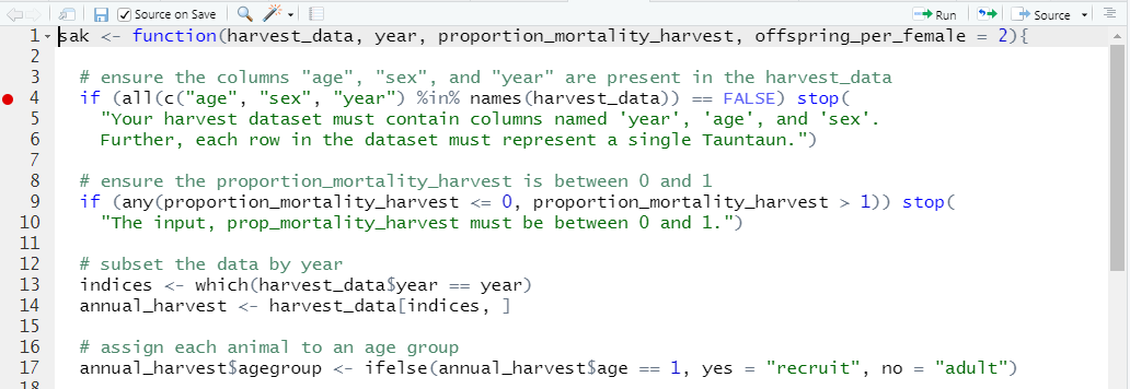
Figure 11.4: Breakpoints in RStudio appear as red dots in the margin.

Here, we’ve placed a breakpoint on line 4 of our SAK function. You should do the same! You may get a message that the breakpoint will be added after the function is re-sourced (in which case, just save your file again if the “source on save” option is checked).

Breakpoints appear as a red dot at the line they will break evaluation. You can add as many breakpoints as you’d like. If you don’t like red dots, breakpoints can be set manually within the SAK function code by inserting setBreakpoint() or browser() at the place where you’d like to break.

Regardless of whether you set a breakpoint in RStudio, or used setBreakpoint() or browser() code within in your SAK code, when the function is called (executed . . . which we’ll do soon), R will enter “browser mode” at the breakpoint, which looks like this:

Figure 11.5: Break mode in RStudio.

The function will run up to the breakpoint, and then stop for evaluation. The line that is waiting patiently to be executed next is highlighted in yellow, and is identified with a little green arrow in the margin.

Look down in the console; debug mode can be identified with the Browse[ ] prompt (more on this later).

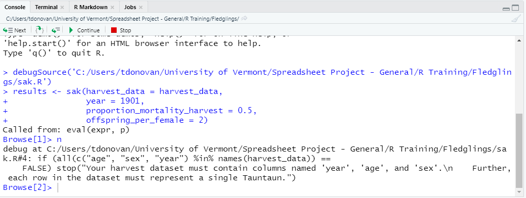
Figure 11.6: When in debug mode, look for the Browse prompt.

If you haven’t done so, go ahead and set a breakpoint towards the top of the body of your sak.R file, save it, and then submit the following code in your console:

# run the SAK function with appropriate arguments
results  <- sak(harvest_data = TauntaunHarvest,
                year = 1901,
                proportion_mortality_harvest = 0.5,
                offspring_per_female = 2)

R should enter break mode as shown in the screen shots above.

When in this interactive mode, you will need to tell R to run the line highlighted in yellow.

We know you are itching to do that, but before we go further, let’s look at your Environment tab. Notice that in break mode, we have now entered the “sak” environment, or the function environment. You should see the objects that were entered as arguments to the SAK function. As you run code in the break (browser) mode, you’ll be working with objects within the function’s environment – not in the global environment. Our function can only “see” the four objects in its function environment.

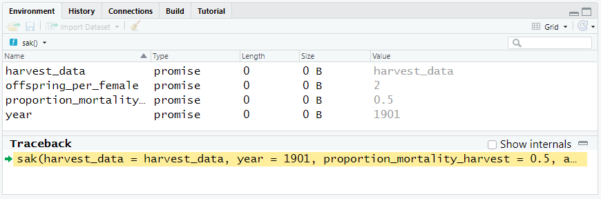
Figure 11.7: When in debug mode, look for the Browse prompt.

The Traceback panel at the bottom indicates which function R is currently working on, and specifies which line number is next up for execution.

We indicated that when you are in browser mode, R is expecting feedback from you on what to do next. Here, the debug buttons in RStudio are useful:

The Next button will run the next line of code.
The button to the right of that will ‘step into the current function call’. This means that if your function calls another function, you can then enter into the second function and step through it.
To the right of that, the button will execute the remainder of the function or loop (handy if you want to ensure the loop works, and want to work through the first few iterations only).
The Continue button will execute the code to the next breakpoint.
The Stop button will take you out of browser() mode. You’ll exit the function environment.

In browser mode, the goal is to make sure that your code works and that R returns objects you need. In browser mode, you can type R commands at will within the console, asking R to return objects within the function environment so that you can verify its value. You can also look in the sak environment pane for changing values of objects.

For non-Rstudio users, once you are in browser mode, you can use several command-line controls which correspond with RStudio’s navigation buttons. The “n” character advances to the next line, the “c” character advances to the end of the flow-control function (so you don’t need to pass through all iterations of a loop, for example), and a capital “Q” ends the debugging browser. If you have an object named “n”, “c”, or “Q” in your function, to identify its value you will need to type print(n), as typing “n” will advance to the next line.

Once you’ve located and fixed your mistakes, you’ll need to clear your breakpoints or delete your calls to setBreakpoint or browser within your code in order for your function to run without interruption. In RStudio, you can quickly clear a single breakpoint by clicking on the red ball again, or you can clear all margin breakpoints (not hard-coded) by going to Debug | Clear All Breakpoints….

Like most things, the best way to learn new tools is to practice.

Exercise:
1. Add three breakpoints to your SAK function.
2. Source your code, and run the function.
3. At the first breakpoint, run the code line by line. Each time, look at what values are stored in the function environment, noting the creation of new objects and changing values of objects.
4. Use your console as your “function sandbox” to find current values of different objects while in debug mode.
5. When you hit your second breakpoint, use the button to advance to the next breakpoint.
6. Finish running out your function and watch for the return to the Global Environment when the function is finished running.

We’ll be using the debug tools again later in this chapter, and getting comfortable with the debug tools will really pay off in the long run. Learn more about debugging in RStudio by going to Debug | Debug help. Also, there is an excellent discussion of debugging in the ebook, What They Forgot to Teach You About R.

11.9 Other Debugging Functions

R has other debugging functions that can be used outside of the RStudio environment and outside of your function script, including: debug(), undebug(), debugonce(), and trace() and traceback(). These functions can be entered into your console directly, and come in handy for those not using RStudio. The function debug() allows the user to step through functions line-by-line every time the function is called, until undebug() is called.

# put the sak function into debug mode
debug(sak)

# run the function; see what happens
results  <- sak(harvest_data = TauntaunHarvest,
                year = 1901,
                proportion_mortality_harvest = 0.5,
                offspring_per_female = 2)

# take the sak function out of debug mode
undebug(sak)

In contrast, debugonce() will step through the function the first time it is called and return to normal operation afterward. This is really helpful because you don’t have to remember to use the undebug function to return to normalcy.

The trace() function and traceback() functions can be used post-mortem – after R tells you an error has been made. These functions will identify the sequence of functions evaluated immediately before the error occurred, so you can see where things went wrong. Our SAK function doesn’t use too many other functions, so let’s try a simple example so you can see traceback in action.

This example is from R’s helpfile on traceback:

# create a function called 'foo'. This function will print the number 1, 
# and execute another function called bar and send it the argument, 2
foo <- function(x) { print(1); bar(2) }

# create a function called bar. This function adds an object that doesn't 
# exist to the input value x
bar <- function(x) { x + a.variable.which.does.not.exist }

# run the function food and pass it the variable 2
foo(2)

[1] 1
Error in bar(2) : object 'a.variable.which.does.not.exist' not found
>

This tells us an error occurred when we tried to run the foo function. But not much else. You can always ask for the call stack by invoking the traceback function after you receive an error:

traceback()

2: bar(2) at #1
1: foo(2)
>

This output is the result of the traceback function. What is shown is called the “call stack”, or a list of function calls made to R. Call stacks are read from the bottom up. In this call stack, we see that the function foo was run with the argument 2 passed into it. R then runs this function: it prints the number 1, and then tries to run the bar function by adding 2 to an object that does not exist. The call stack ends with the bar function, so you know where the error occurred. Of course, if you happened to have an object in your environment called a.variable.which.does.not.exist that was a number, you would not get this error!

The call stack will show you which function caused the problem. This is a very important tool for debugging, especially when functions use multiple other functions.

For a one-stop-shop on debugging methods, see Rob Hindman’s web page on debugging in R. Also check out the package testthat, “a testing package specifically tailored for R that’s fun, flexible and easy to set up.”

11.10 Using a Function Repeatedly

Hopefully you have been successful in getting your SAK function to run an analysis. Remember, this function (by design) estimates population size one year at a time. But what if you want to use this function to evaluate population size for multiple years? Or what if you want to determine how ‘sensitive’ the output is to changes in a particular input? There are several options, and here we’ll take some time to introduce the concept of vectorization in R, introduce loops, and introduce the lapply function.

11.10.1 Vectorization in R

We’ve been running the SAK with the following inputs:

sak(harvest_data = harvest_data,
                year = 1901,
                proportion_mortality_harvest = 0.5,
                offspring_per_female = 2)

## $`Total Population Estimate`
## [1] 6242.6
## 
## $`Harvest Rate`
## [1] 0.3061224
## 
## $`Total Male Adult Estimate`
## [1] 1440.6
## 
## $`Total Female Adult Estimate`
## [1] 1600.667
## 
## $`Total Offspring Estimate`
## [1] 3201.333

But what if we were unsure about the input, proportion_mortality_harvest, or some other input? We could run the analysis again by setting this input to 0.25, and comparing the new result with the original one.

sak(harvest_data = harvest_data,
                year = 1901,
                proportion_mortality_harvest = 0.25,
                offspring_per_female = 2)

## $`Total Population Estimate`
## [1] 12485.2
## 
## $`Harvest Rate`
## [1] 0.1530612
## 
## $`Total Male Adult Estimate`
## [1] 2881.2
## 
## $`Total Female Adult Estimate`
## [1] 3201.333
## 
## $`Total Offspring Estimate`
## [1] 6402.667

Here, we can see that the first analysis returns an estimate of 6242.6 while the second analysis returns an estimate of 6242.6.

A cool feature of our function is the capability to allow proportion_mortality_harvest to ingest several inputs for this argument. Let’s illustrate this by creating a vector that stores inputs for proportion_mortality_harvest, and then pass the function this vector as follows:

# create a vector with varying inputs for proportion.mortality.harvest
range.proportion.mortality.harvest <- c(0.25, 0.5, 0.75)

results <- sak(harvest_data = TauntaunHarvest,
                year = 1901,
                proportion_mortality_harvest = range.proportion.mortality.harvest,
                offspring_per_female = 2)

# show the results
results

## $`Total Population Estimate`
## [1] 12485.20  6242.60  4161.73
## 
## $`Harvest Rate`
## [1] 0.1530612 0.3061224 0.4591837
## 
## $`Total Male Adult Estimate`
## [1] 2881.2 1440.6  960.4
## 
## $`Total Female Adult Estimate`
## [1] 3201.333 1600.667 1067.111
## 
## $`Total Offspring Estimate`
## [1] 6402.667 3201.333 2134.222

Wow! We didn’t expect our function could do this! What a nice surprise! This time, we got three estimates for each portion of output, the first corresponding with proportion_mortality_harvest = 0.25 and the last third corresponding with proportion_mortality_harvest = 0.75. You can see that the total population estimate is quite sensitive to changes in the input, proportion_mortality_harvest. When the rate is 0.25, the total population estimate is 12485.2, whereas the estimate is 4161.73 when the rate is 0.75.

Why does our function produce three outputs?

To see why, debug!

Exercise:
1. To see what’s going on, clear all breakpoints in your SAK function.
2. Then insert a single breakpoint into your function towards the top of the function.
3. Then run the code again in debug mode. Remember that you’ve passed in a vector of values for the argument, proportion_mortality_harvest.
4. Things get interesting at the line:
harvest_rate <- annual_mortality_rate * proportion_mortality_harvest
5. After this line is run, use your console to double-check your results line by line. That is, run the line of code, then use your console to show it so you can see what the object currently looks like.

The key here is the ordering of operations within the function body. By the time the proportion_mortality_harvest is used, we have already calculated the adult male harvest rate. The next line multiplies the harvest_rate (a vector with one element) by proportion_mortality_harvest (a vector with three elements), so R uses its vectorization methods to compute the remaining calculations, which allows R to run all three analyses simultaneously. Double check the calculations as you continue line by line through the code, checking on object values in your console. No loop is needed!

It’s very instructive to test a function in debug mode to find out how the function behaves in a step-by-step manner.

Will this vectorization work for the year argument too? Let’s try it by entering both 1901 and 1902 for the year argument:

results_combined <- sak(harvest_data = TauntaunHarvest,
                year = c(1901, 1902),
                proportion_mortality_harvest = 0.5,
                offspring_per_female = 2)

# show the object
results_combined

## $`Total Population Estimate`
## [1] 7311.68
## 
## $`Harvest Rate`
## [1] 0.2576832
## 
## $`Total Male Adult Estimate`
## [1] 1641.55
## 
## $`Total Female Adult Estimate`
## [1] 1890.042
## 
## $`Total Offspring Estimate`
## [1] 3780.084

Surprisingly, the function does not stop, but it returns result. How does this result compare to a function call where year is 1901? 1902?

# run the analysis for the 1901 data
results_1901 <- sak(harvest_data = TauntaunHarvest,
                year = 1901,
                proportion_mortality_harvest = 0.5,
                offspring_per_female = 2)

# show the results
results_1901

## $`Total Population Estimate`
## [1] 6242.6
## 
## $`Harvest Rate`
## [1] 0.3061224
## 
## $`Total Male Adult Estimate`
## [1] 1440.6
## 
## $`Total Female Adult Estimate`
## [1] 1600.667
## 
## $`Total Offspring Estimate`
## [1] 3201.333

# run the analysis for the 1902 data
results_1902 <- sak(harvest_data = TauntaunHarvest,
                year = 1902,
                proportion_mortality_harvest = 0.5,
                offspring_per_female = 2)

# show the results
results_1902

## $`Total Population Estimate`
## [1] 11470.08
## 
## $`Harvest Rate`
## [1] 0.1940701
## 
## $`Total Male Adult Estimate`
## [1] 1911.681
## 
## $`Total Female Adult Estimate`
## [1] 3186.134
## 
## $`Total Offspring Estimate`
## [1] 6372.269

Hmmmm. The 1901 analysis returned an estimate of 6242.6, while the 1902 analysis returned an estimate of 11470.08. The combined analysis returned an estimate of 7311.68. What exactly is returned with our attempt at sending in two years? Debug!

Exercise:
1. To see what’s going on, clear all breakpoints in your SAK function.
2. Then insert a single breakpoint into your function towards the top of the function.
3. Then run the code again in debug mode. Remember that you’ve passed in a vector of values for the year argument.
4. Things get interesting at the line indices <- which(harvest_data$year == year) and annual_harvest <- harvest_data[indices, ]
5. After this line is run, use your console to double-check your results line by line. That is, run the line of code, then use your console to show it so you can see what the object currently looks like.

What did you learn? Inside the sak function, the object, indices returns all harvest records in 1901 and 1902. Perhaps this is what you wanted. Or perhaps you wanted the results to be returned by year? If the latter, clearly a different approach will be needed!

11.10.2 For Loops

If we are interested in evaluating a series of inputs for year in our sak function, we can use a for loop in R.

All computer languages have mechanisms for repeating a block of code over and over again until a stopping rule is encountered. R offers a handful of loop options. If we wanted the loop to iterate until a certain criterion is met, we would use a while loop. However, in our Tauntaun SAK analysis, we know we want to generate results for two years. Thus, we can define exactly how many iterations we need the loop to pass through. To do this, we use a for loop. In R, the syntax for a for loop is:

for (i in vector){

  do something
  
}

Let’s look at a for loop in action.

# look at the built-in vector called letters
letters

##  [1] "a" "b" "c" "d" "e" "f" "g" "h" "i" "j" "k" "l" "m" "n" "o" "p" "q" "r" "s" "t" "u" "v" "w" "x" "y" "z"

# allocate an empty vector that will store results of the loop
output <- vector(length = length(letters), mode = "character")

# loop through each element of numbers, and add the number 1 to it
for (i in 1:length(letters)) {
  output[i] <- paste(letters[i], "_out")
}

# look at the object, numbers
output

##  [1] "a _out" "b _out" "c _out" "d _out" "e _out" "f _out" "g _out" "h _out" "i _out" "j _out" "k _out" "l _out" "m _out" "n _out" "o _out" "p _out"
## [17] "q _out" "r _out" "s _out" "t _out" "u _out" "v _out" "w _out" "x _out" "y _out" "z _out"

The for loop has the following code structure:

the word “for” starts the loop
this is followed by a set of parentheses, inside of which there is an identifier that identifies the loop number. Here, we named our identifier i (for iteration). We could have named it something more descriptive if we wished. The code, i in 1:length(letters) means we’ll let i take on the values 1 through however many letters there are. When the loop starts, a new variable called i will be created, and it will have a value of 1.
this is followed by a set of braces { }, inside of which is code that specifies what to do. Here, we’ll take the the vector, letters, and we’ll extract the i^{th} element from it and paste "_out" to the end of it. For example, if we are on loop # 4 (i = 4), we’ll extract the fourth element from letters (d) and paste "_out" to it, creating the output “d_out” as the fourth element of the results vector.

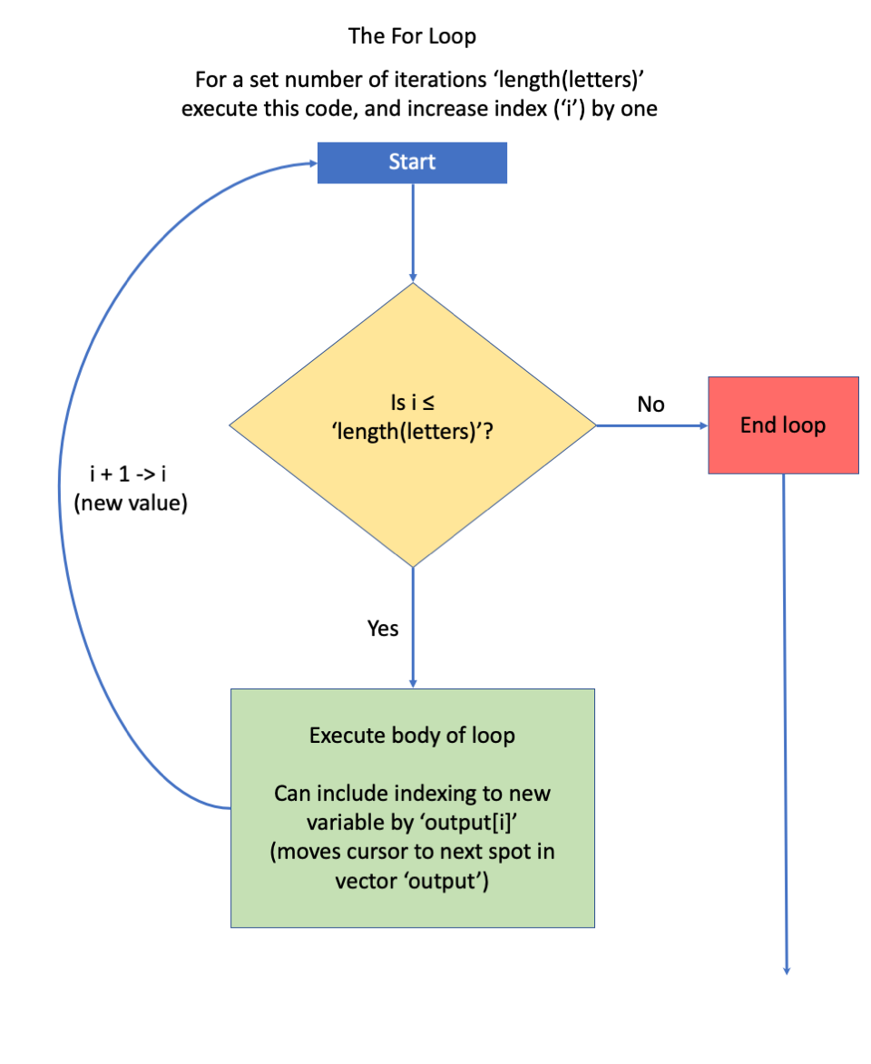
Figure 11.8: Box diagram courtesy of Jacob Weissgold.

Let’s try it with the SAK function, with the code provided in the code chunk below. Let’s walk through this code first. See if you can find these elements in the code below:

First, we’ll set up a vector of values called yrs, which holds the two years we are interested in evaluating.
Then, we’ll create an empty list called sak.results, which will be a list that stores the results of each year. This might sound confusing, especially if you remember that our SAK function output is a list as well. If the sak output is a shoestore containing different objects (shoes) that give a certain kind of output, our sak.results list will be a shopping outlet mall that has multiple shoestores!
Then, we’ll start the for loop by entering for (y in 1:length(yrs)). This code identifies the name of our counter, y, and indicates that a will take on values from 1 to the length of our yrs vector, which is 2.
Inside the braces, we’ll run the SAK function. When the code is first run, y will take on the value 1 in the loop. The year argument for the sak function will be set to year = yrs[y]. What’s going on here? Well, if y == 1, then R will take the first element of your yrs vector, which is 1901. In our first pass through, y == 1, so the the year argument will be 1901.
After the first SAK call is executed, the output will be stored in the appropriate section of the sak.results list.
In the second pass of our loop, y will take on the value of 2. The year argument for the sak function will be set to year = yrs[y]. If y == 2, then R will take the second element of your yrs vector, which is 1902.

Clear all breakpoints from your SAK function, and run this code now in your chapter11.R script!

# set up a vector of years for analysis
yrs  <- c(1901, 1902)

# create an empty list to store the output
sak.results <- list()


for (y in 1:length(yrs)) {
  
  # run the sak function using this new vector as an input
  results <- sak(harvest_data = TauntaunHarvest,
                year = yrs[y],
                proportion_mortality_harvest = 0.5,
                offspring_per_female = 2)
  
  # write your results from this iteration to the sak.results list.
  sak.results[[y]]  <- results
  
  # name the list element the year; this will be a character
  names(sak.results)[[y]] <- yrs[y]
  
  } # end of for loop

# look at the list
str(sak.results)

## List of 2
##  $ 1901:List of 5
##   ..$ Total Population Estimate  : num 6243
##   ..$ Harvest Rate               : num 0.306
##   ..$ Total Male Adult Estimate  : num 1441
##   ..$ Total Female Adult Estimate: num 1601
##   ..$ Total Offspring Estimate   : num 3201
##  $ 1902:List of 5
##   ..$ Total Population Estimate  : num 11470
##   ..$ Harvest Rate               : num 0.194
##   ..$ Total Male Adult Estimate  : num 1912
##   ..$ Total Female Adult Estimate: num 3186
##   ..$ Total Offspring Estimate   : num 6372

Here, you can see a list of two is returned, one for each year of interest.

Now that you have a sense of where we’re headed, let’s run this code once more, but add a breakpoint somewhere towards the top of the sak function’s body (and re-source it).

Exercise:
1. Run the code above in break mode, clicking line by line through the code.
2. Check out what R thinks y is when you are in break mode, and check the objects within the function environment each time a new line is submitted.
3. When you get to the end of the first loop, check the sak.results list and see how the first loop’s analysis is stored.
4. Continue clicking the run next line button, and work your way through the next loop.
5. Remember you can use your console to check the values of objects when you are in break mode. It’s useful to type in the letter y to find the index value.

Break mode is a powerful way to build a good understanding of loops (and many other tricks in R!).

11.10.3 The Apply Functions

R has other ingenious ways of looping that do not involve an actual loop. These are collectively known as the “apply” functions, and in some cases they are “speedier” than for loops. Each function is designed to “do something” over each element of an object (a list or vector), but they vary in the type of object that is returned.

We’ve touched on the apply functions in previous chapters, but it never hurts to review. From the help files, we learn that:

lapply returns a list of the same length as X, each element of which is the result of applying FUN to the corresponding element of X
sapply is a user-friendly version and wrapper of lapply by default returning a vector, matrix or, if simplify = “array”, an array if appropriate
vapply is similar to sapply, but has a pre-specified type of return value, so it can be safer (and sometimes faster) to use
mapply mapply is a multivariate version of sapply
tapply applies function to each cell of a ragged array, that is to each (non-empty) group of values given by a unique combination of the levels of certain factors.
rapply is a recursive version of lapply

While each function has its nuances, they share a similar call structure, which makes learning to use them more straightforward. These functions share two arguments, X and FUN, and they all apply the function defined in the FUN argument to all levels of X.

Let’s look at a helpfile:

help(lapply)

Here, we see that “lapply returns a list of the same length as X, each element of which is the result of applying FUN to the corresponding element of X.”

In the Usage section of the helpfile, we see the common use of lapply looks like this:

lapply(X, FUN, . . .)

X is the object to loop over, and FUN is the function to use. What are the three dots? The function lapply has two arguments and some dots: lapply(X,FUN, . . . ). The dots are where you specify the arguments corresponding with the particular FUN you want to use.

If we’re going to use lapply, we need to first make sure that our object, X, is a list where each section of the list can have a function applied to it. In Chapter 4, we used lapply over different columns of a data frame to find the class. This works because a data frame is a list of different vectors, all of the same length. Let’s refresh our memory:

lapply(X = TauntaunHarvest, FUN = class)

## $hunter.id
## [1] "numeric"
## 
## $age
## [1] "numeric"
## 
## $sex
## [1] "factor"
## 
## $individual
## [1] "numeric"
## 
## $species
## [1] "character"
## 
## $date
## [1] "Date"
## 
## $town
## [1] "factor"
## 
## $length
## [1] "numeric"
## 
## $weight
## [1] "numeric"
## 
## $method
## [1] "factor"
## 
## $color
## [1] "factor"
## 
## $fur
## [1] "factor"
## 
## $month
## [1] "numeric"
## 
## $year
## [1] "numeric"
## 
## $julian
## [1] "numeric"
## 
## $day.of.season
## [1] "numeric"
## 
## $sex.hunter
## [1] "factor"
## 
## $resident
## [1] "logical"
## 
## $count
## [1] "numeric"

If we want to run the sak function by year, we need to provide the lapply function a list in which the SAK can be applied to each section of the list. To do that, we’ll first use the split function to create a list called data.list, splitting the harvest dataset by year.

# split the harvest data frame into sections by year
data.list  <- split(x = TauntaunHarvest, f = TauntaunHarvest$year)

# verify what's inside the object, data.list
str(data.list, max.level = 1)

## List of 10
##  $ 1901:'data.frame':	931 obs. of  19 variables:
##  $ 1902:'data.frame':	900 obs. of  19 variables:
##  $ 1903:'data.frame':	1118 obs. of  19 variables:
##  $ 1904:'data.frame':	1255 obs. of  19 variables:
##  $ 1905:'data.frame':	1359 obs. of  19 variables:
##  $ 1906:'data.frame':	1433 obs. of  19 variables:
##  $ 1907:'data.frame':	1506 obs. of  19 variables:
##  $ 1908:'data.frame':	1560 obs. of  19 variables:
##  $ 1909:'data.frame':	1616 obs. of  19 variables:
##  $ 1910:'data.frame':	1674 obs. of  19 variables:

Let’s now look at the dots argument in action. Here, we will use the lapply function to provide the first record of each element in our data.list. Notice that we provide FUN = head to specify that we want to use the head function, but we also pass in the arguments to the head function, specifically n = 1:

results  <- lapply(X = data.list, FUN = head,  n = 1)
# look at the results
results

## $`1901`
##       hunter.id age sex individual  species       date    town length   weight     method color  fur month year julian day.of.season sex.hunter
## 10600       560   1   f        116 Tauntaun 1901-10-01 ADDISON 294.35 677.1833 lightsaber White Long    10 1901    274             1          m
##       resident count
## 10600    FALSE     1
## 
## $`1902`
##       hunter.id age sex individual  species       date       town length   weight method color    fur month year julian day.of.season sex.hunter
## 11740       616   1   f       1167 Tauntaun 1902-10-01 CHARLESTON 301.16 761.1551 muzzle  Gray Medium    10 1902    274             1          m
##       resident count
## 11740    FALSE     1
## 
## $`1903`
##       hunter.id age sex individual  species       date   town length   weight     method color  fur month year julian day.of.season sex.hunter
## 11696       614   1   f       2046 Tauntaun 1903-10-01 BOLTON 301.89 906.0901 lightsaber White Long    10 1903    274             1          m
##       resident count
## 11696     TRUE     1
## 
## $`1904`
##      hunter.id age sex individual  species       date       town length   weight method color    fur month year julian day.of.season sex.hunter
## 6739       352   1   f       3126 Tauntaun 1904-10-01 BENNINGTON 314.99 906.5457    bow  Gray Medium    10 1904    275             1          m
##      resident count
## 6739     TRUE     1
## 
## $`1905`
##       hunter.id age sex individual  species       date       town length   weight method color  fur month year julian day.of.season sex.hunter
## 13094       687   1   m       4631 Tauntaun 1905-10-01 BENNINGTON 406.96 973.8766    bow  Gray Long    10 1905    274             1          m
##       resident count
## 13094     TRUE     1
## 
## $`1906`
##      hunter.id age sex individual  species       date    town length   weight     method color   fur month year julian day.of.season sex.hunter
## 6146       320   2   m       6464 Tauntaun 1906-10-01 ANDOVER 351.64 970.0472 lightsaber  Gray Short    10 1906    274             1          f
##      resident count
## 6146    FALSE     1
## 
## $`1907`
##      hunter.id age sex individual  species       date    town length   weight method color    fur month year julian day.of.season sex.hunter resident
## 1576        84   3   m       8259 Tauntaun 1907-10-01 ADDISON 524.13 1326.978    bow White Medium    10 1907    274             1          f     TRUE
##      count
## 1576     1
## 
## $`1908`
##      hunter.id age sex individual  species       date   town length   weight method color  fur month year julian day.of.season sex.hunter resident
## 4253       223   1   f       8729 Tauntaun 1908-10-01 ALBANY 308.72 803.3434 muzzle  Gray Long    10 1908    275             1          m     TRUE
##      count
## 4253     1
## 
## $`1909`
##      hunter.id age sex individual  species       date      town length   weight method color    fur month year julian day.of.season sex.hunter
## 5233       274   1   f      10283 Tauntaun 1909-10-01 ARLINGTON 265.18 594.4567 muzzle  Gray Medium    10 1909    274             1          m
##      resident count
## 5233     TRUE     1
## 
## $`1910`
##      hunter.id age sex individual  species       date   town length  weight     method color    fur month year julian day.of.season sex.hunter
## 6956       366   1   f      11810 Tauntaun 1910-10-01 BERLIN 297.16 577.087 lightsaber  Gray Medium    10 1910    274             1          f
##      resident count
## 6956     TRUE     1

Now, can we use the lappy function to look through our sak function? Let’s try it:

results  <-  lapply(X = data.list, FUN = sak,  
                proportion_mortality_harvest = 0.5,
                offspring_per_female = 2)

Error in which(harvest_data$year == year) : argument "year" is missing, with no default

What happened here? Well, our sak function has a year argument, which is required but has no default value. We need to find a way a way to pass the year argument. We can do that with the mapply function. Let’s have a look at this helpfile:

help("mapply")

Here, the description tells us that “mapply is a multivariate version of sapply. mapply applies FUN to the first elements of each … argument, the second elements, the third elements, and so on. Arguments are recycled if necessary.” Let’s try it. We need to send mapply a vector named year which can be used by our sak function:

mapply(data.list, FUN = sak, year = 1901:1910, 
                proportion_mortality_harvest = 0.5,
                offspring_per_female = 2)

##                             1901      1902      1903     1904      1905      1906      1907      1908      1909      1910     
## Total Population Estimate   6242.6    11470.08  5198.39  6972.25   8227.6    9160.66   10168.81  10528.78  10857.64  11249.42 
## Harvest Rate                0.3061224 0.1940701 0.322898 0.2874251 0.2708333 0.2627646 0.2520468 0.2519774 0.2527293 0.2526371
## Total Male Adult Estimate   1440.6    1911.681  1731.197 2324.083  2747.077  3055.967  3392.227  3512.22   3624.432  3752.418 
## Total Female Adult Estimate 1600.667  3186.134  1155.73  1549.389  1826.84   2034.897  2258.861  2338.855  2411.069  2499     
## Total Offspring Estimate    3201.333  6372.269  2311.459 3098.778  3653.68   4069.795  4517.723  4677.71   4822.138  4998.001

Cool! We’ve used the mapply function to run our sak function for each year without a loop. With R, you will want to have both “for loops” and a handful of “apply” functions in your back pocket to help automate an analysis repeatedly.

11.11 Next Steps

Gold stars all around! Don’t feel overwhelmed by all content in this chapter. It takes practice to create functions, and to become comfortable with debugging. But, if you have tasks that repeatedly do as part of your job, it may well be worth the time and effort to create functions that automate this work.

Now that you’ve made two functions, we’ll learn how to put them into an R package so that you can give it to your Tauntaun colleagues. Our function inputs are tricky enough that we’ll want to make sure that our helpfiles are well-written and will help our Tauntaun colleagues use them correctly. In the next chapter, you will learn how to build a package using tools in RStudio.

11.12 References

References

Gove, Nancy, John Skalski, Peter Zager, and Richard Townsend. 2002. “Statistical Models for Population Reconstruction Using Age-at-Harvest Data.” The Journal of Wildlife Management 66: 310–20. https://doi.org/10.2307/3803163.