Chapter 2 A Brief Tour of RStudio
In this chapter, we’ll take a quick spin through RStudio. Along the way, you will be creating your first R script. The developers of RStudio provide fantastic documentation on their website, and it is worth exploring this site at your leisure. The intention here is to give you a big overview rather than poking through each and every option (we’ll introduce the various options and settings as we work through our Tauntaun exercise).
When you open R Studio for the very first time, you’ll see three panes on your screen. After you’ve written one script (later in this chapter!), you’ll see four panes. These are, starting in the upper left, the (1) source editor, also called the script editor; (2) the workspace and history pane; (3) the R console, and 4) the files, plots, packages, and help pane.
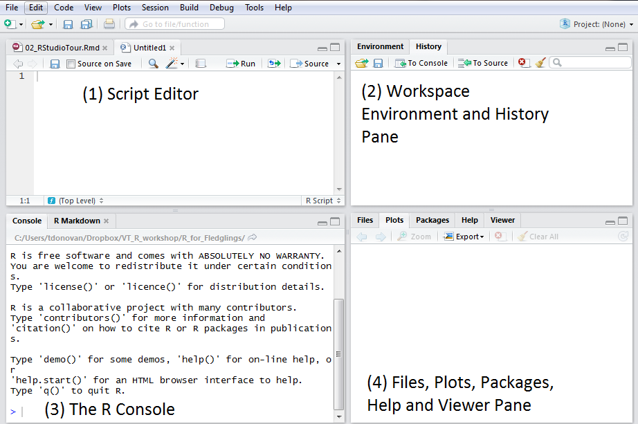
Figure 2.1: The RStudio panes.
Let’s look at each of these panels in more detail, starting with the R Console.
2.1 The R Console
The R console (located in the lower left pane of RStudio) is where commands are submitted to R to execute.

Figure 2.2: The console.
When you first open R, the console provides you with information on which version of R you are currently running. R is updated twice a year….more often than this book is updated! It’s generally best to use the most up-to-date program in your work.
The version information in the console is followed by some example commands you may wish to submit. Type your commands after the prompt symbol, which looks like this:
>
You should see a vertical, blinking bar to the right of the prompt, which is where you start typing.
What exactly will you be typing? Generally speaking, you’ll enter commands into the console that either:
- Run a function, or
- Create or modify an object.
We’ll cover both of these concepts in great detail in later chapters, but for now type in the sqrt(10) into your Console (or copy and paste it into the Console), and then hit return.
## [1] 3.162278Throughout this book, you will be entering R code into a script or the console. The R code is shown in shaded blocks in the document, and can be copied and pasted if desired. We’ll show you R’s response in a separate block that contains double-hash tags (##). These double-hash tags won’t appear in your output – we’ve added it here to clearly separate the R input from the R output.
You’ve just used one of R’s functions called sqrt and passed the value 10 to it. This means that you want R to evaluate the square root of 10. The answer is 3.162. You may have more or fewer decimals….don’t worry about that for now. Also, we’ll cover what the [1] in the output means later.
Now try typing in Sqrt(10) in your console:
Error in Sqrt(10) : could not find function "Sqrt"The important take-home point here is that R is case sensitive. Never forget this!
2.2 The Editor Pane
Normally, you would not interact directly with the Console, but instead would type your code into a “script file”, and then “send” the code from the script to the console, where R will execute it. The script file will be your long-term record of what code you ran; the console will only keep a short-term record of it (which can be accessed using the up-arrow).
If you type commands into the Console, but don’t save them in your script, those commands will be lost to future R sessions unless you take actions to save your R history (described later).
Let’s create our first script. In RStudio, go to main toolbar, and choose File | New File | R Script. You should see a blank document in the upper left panel of RStudio.
Type (or copy) the following two lines of code (shown in the gray box below), and paste it into your new script.
In R, lines of code that are preceded by the # symbol are considered “comments”. So get the square root of 10 is a comment. Make sure to paste in the comments too!
Comments are not actually executed in R – they are notes that you (the coder!) type to remind yourself of what the code is intended to do. Notice that this font is green (by default) in RStudio; this helps you quickly differentiate between comments and code. (These color schemes don’t appear in this ebook).
To send code to R, place your curser anywhere on the line to be executed, then press the Run button  in the upper right hand portion of your screen. You should notice that your curser dropped down to the next line.
Instead of running one line at a time, you can select the entire block with your mouse (comment and all), and then press Run. This approach is useful to sending multiple commands to R at once.
If you don’t like moving your mouse to the Run button, you can use Ctrl + Enter (PCs) or Command + Return (Macs) to submit a line or selection. Try it! All of the shortcuts in RStudio can be found under Help | Keyboard Shortcuts.
Exercise:
- Create a directory (folder) on your C drive or somewhere convenient on your computer, and name it “R_for_Fledglings”. We use Windows, and our directory is located on the C drive. If you are on a Mac, create this folder in your user profile (find the house icon in your Finder menu, click it, and then create the directory there). Like most computer naming conventions, it’s best to avoid spaces. The specific location is not relevant as long as you know where it is.
- Save the script file that you have just created to your new directory, and name it “chapter2.R”.
- Close RStudio. If by chance you are prompted as to whether to save the workspace image, select “Don’t Save” (otherwise all of the objects in your Global Environment will be saved for later use – there’s no need for this now).
- Navigate to your file, chapter2.R and double click on it. This file should open in RStudio. If it opens with another program, right click on the file and see if you can set the “open with” default to RStudio.
- Explore the other options in the Editor pane….we’ll be using them later on but take a sneak peak for now.
Why type your code in script files and not directly in the console? There are two good reasons. First, you’ll make lots of mistakes when you code, and really only want to keep the code that works exactly as intended. In other words, a good practice is to save the script file (cleaned of any coding mistakes), and then just run the script to re-create things when you want them. Second, if you code a lot, you’ll find that you can re-use bits of code from a previous analysis. This saves you from having to re-create the wheel from scratch.
When you re-open your document chapter2.R in RStudio, you should see the following in the Script pane:
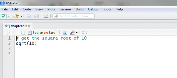
Figure 2.3: The file, chapter2.R, in RStudio’s editor pane.
Notice that the tab with the name chapter2.R is activated, and you can see the code as well. Now you’re free to execute your code once more (you really want that square root of 10!).
2.3 The Files, Plots, Package, Help Pane
2.3.1 The Files Tab
Now let’s shift our attention to RStudio’s lower right pane. When you opened chapter2.R again, something new appeared in the Files tab in the lower right hand pane. Do you see the file called chapter2.R? If you don’t see it, try hitting the refresh button, which looks like this: 
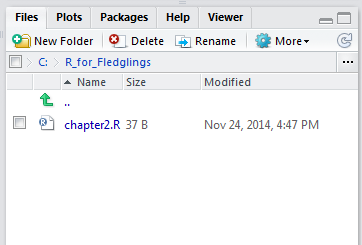
Figure 2.4: The files tab.
Notice the file path C:R_for_Fledglings. This means that our R_for_Fledglings directory is a folder in the C drive….keep that in mind as we go along. Your path may differ.
The Files tab lets you create new folders (directories) on your computer, as well as move, delete, and rename files. In RStudio, you can navigate to anywhere on your computer by clicking on the three dots in the upper right hand corner of the Files pane 
When you open an existing script, the directory that houses your R script file will automatically appear in the Files list. If you add new files, rename files, or delete files, you may need to refresh this list so that RStudio is showing the most up-to-date view of files:
The “More”" button in the Files tab is another handy feature. Click on it and you’ll see the following:
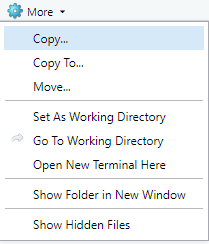
Figure 2.5: The More button.
When you are working in R, the program needs to know where to find inputs and deliver outputs, and will look first in what is called a “working directory”. You can find your working directory by using the getwd function, which can be entered in your console or in your script:
If you’re using Windows, you may see this response:
"C:/R_for_Fledglings"If you’re using a Mac or Linux, you may see a response like this:
"~/[username]/R_for_Fledglings"Generally speaking, when you are working on a project, you will want to organize all of the files for a given project in one folder, and that particular folder should be established as your working directory. This would include the script files, any images that you create in R, the datasets or csv files that you call into R for analysis, etc. It’s a good idea to check what R thinks is your working directory at the beginning of each R session.
What if you want to change the working directory? By clicking More button, and then the option Set As Working Directory, you force the folder that contains your file, chapter2.R to be your working directory.
Alternatively, you can set the working directory by using the setwd function in R. If your directory R_for_Fledglings was placed on your C drive, for example, you can set the working directory like this (note: Mac users will have a different file path):
# use the setwd() function to set the working directory
# notice the forward slashes used to separate levels
setwd("C:/R_for_Fledglings")
If you use this option, you’ll need to be able to write out the filepath, which can be hard to remember. R has two handy functions for Windows users that return the filepath to a directory (folder) or file: choose.dir and choose.files. Mac, Linus, and Windows users can use the file.choose function to return the filepath of a selected file. These functions open a new window that allows you to browse to a file or directory of choice.
Copy the code below into your script that pertains to the operating system you use.
# PC users should be able to run these lines of code

# navigate to a folder or directory on your computer
choose.dir()

# navigate to a particular file on your computer
choose.files()

################################################################

# Mac, Linux, and Windows users should be able to find a file with file.choose()

file.choose()
2.3.2 The Help Tab
The Help tab in the lower right hand pane is another super useful feature of RStudio. If you know the name of the function you want some help with, you can use the help function to bring up the helpfile for that function. Let’s find the helpfile for the sqrt function. Copy the following code into your script, and then run it.
The Help tab now displays the helpfiles for the sqrt function. Your web browser may have also opened up to display the helpfile. Scan through the helpfile to get a sense of what information is displayed there.
If there is a function called meatloaf, you can get help on the function by typing in help(meatloaf). R would bring up the help file for the meatloaf function. A shortcut for the word “help” is a question mark. So ?meatloaf does the same thing.
But what if you don’t know a function’s name, or are looking for help on something other than a function? First, try using the single question mark notation or help function:
## No documentation for 'meatloaf' in specified packages and libraries:
## you could try '??meatloaf'
Here, R does not find documentation for meatloaf and suggests that you use the double question mark approach, which would be ??meatloaf. This invokes a keyword search. The double question mark is actually a shortcut for the function help.search. Two question marks means “search the entire R repository for a key word”. If you use the help.search function, be sure to include your search word in quotes:
Oh well….maybe some day there will be a meatloaf function in R!
Exercise:
Below are a few common functions that you might have used in Excel if you are a spreadsheet user. We list the familiar names of the functions Excel uses to take an average (‘average’), compute the standard deviation (‘std’), find a value in a range specified cells (‘index’), calculate the sum (‘sum’) or find the minimum value (‘min’) for a range of cells. R has functions that do these things too, but the names of the functions may be different! Try the help, ?, help.search, and ?? approaches. Failing those, try Google.
- average (a tricky one; this is the arithmetic mean)
- std (another tricky one; this is the standard deviation)
- match (find a particular value in a column of cells, and return its position)
- sum
- min
The answers are provided at the end of this chapter (but don’t cheat….you’ll learn a lot more about R by working through exercises on your own!)
2.3.3 The Plots Tab
The Plots tab holds all of the plots you may create in your R session. To demonstrate this, let’s use the help function and find more information about a function called plot.
If you’ve installed other packages, you may see that the plot function is used by several different packages. Here, we are interested in “Generic X-Y Plotting” for base R.
Each helpfile in R contains a section called Examples, and there you can copy code from the helpfile and run it in the console to see an example of the function in action. Scroll down the plot helpfile and copy the following lines of code from the plot helpfile into your R script file. Then paste the code to the R console and press enter:
Figure 2.6: Plot generated by R’s plot function.
Don’t worry about interpreting the code for now. We just want you to know that the plot you created is stored in the Plots tab.
We can run the other examples from R’s plot helpfile with the handy example function:
When you use the example function, R will execute the examples from the helpfile so you don’t need to type anything. Did you notice that R returned “Hit plot function are run, generating several plots. You can “scroll” through them by pressing the arrow buttons located in the Plots tab 
Like other tabs we’ve seen, the Plots tab has several buttons at the top that let you zoom into an image, export the image, delete the image, or clear all images by clicking on the broom icon 
Save your file before doing the next set of exercises.
Exercise:
- Click on an image, then click on the zoom button.
- Export your image as an image or pdf to your working directory.
- Click the refresh button to update your files.
- Locate the image in the Files tab and view it by clicking on it.
- After you have finished with #4, delete the image.
- Comment out ALL of your code except the line that reads plot(x <- sort(rnorm(47)), type = “s”, main = “plot(x, type = "s")”). This can be done by selecting all lines except the line of interest, then going to Code | Comment/Uncomment Lines.
- Close RStudio. If prompted as to whether to save the workspace image, select “Don’t Save”.
- Reopen your file.
- Run your code once more. Instead of clicking through the R code line by line (with the Run button), run the entire script by pressing the source button.
The source button looks like this: 
You should see a similar result as below:
Figure 2.7: Sourcing a file will run the full script.
In the upper left pane, the tab for your file chapter2.R is activated and showing the code. As with most things in RStudio, any time you press a button, an R function is invoked. In this case, the “source” button runs the source function. Look at this function’s helpfile, and you’ll see its description: “source causes R to accept its input from the named file or URL or connection or expressions directly. Input is read and parsed from that file until the end of the file is reached, then the parsed expressions are evaluated sequentially in the chosen environment.”
We will use the source button in chapter 9.
Exercise:
- Uncomment your comments by going to Code | Comment/Uncomment lines.
- Submit your code line by line (instead of sourcing it). You can do this by selecting all text and then pressing Run.
As a result of sourcing your code or submitting it line by line, R produced some new items of interest. This brings us to to our last pane in our tour of RStudio, the Environment and History Pane (yours may look a bit different than ours depending on what code you have submitted).
2.4 The Environment and History Pane
2.4.1 The History Tab
In the upper right pane of R Studio, you’ll see the Environment and History pane. Click on the History tab, and you should see a history of all of the commands that you have sent to the R console in this session.
Figure 2.8: Notice the code in the History tab.
A few things are worth noting about history:
- When you open an R script or create a new R script, R automatically creates a file called .Rhistory, and writes the commands to this file so you can retrieve it later if you wish. This is raw, unedited code; some of it may generate mistakes, and some may not!
- You can save your history by pressing the save icon in the History tab. The .Rhistory file would then contain all of your commands (and be greater than 0 bytes).
- You can clear the history by pressing the broom icon in the history window.
- You can also get this history by typing history() in the R console, which calls up a function called
history. - In the History tab, you can select a given line, then press the “To Console”" icon to send old code back to the console.

- In the R console itself, you can use your up and down arrow keys to find recently submitted commands.
2.4.2 The Environment Tab
Now let’s click on the Environment tab, which is the Most Valuable Player (MVP) of RStudio if you are a fledgling. You should see that R has created an object called “x”. Where did this come from? You created this when you copied and ran the code from the sqrt function helpfile. It’s too soon in this book to understand this object in depth, so let’s create another object that is easier to grasp.
Earlier we used the sqrt function to calculate the square root of a number. That was neat, but it would be nice to save the result for later. Let’s do that now, and create an object called “result”. Type in the following in your script:
# use the sqrt function to calculate the square root of 10
# store the result in an object called "result"
result <- sqrt(10)
Now you should see that the object appears in the section on the Environment tab labeled “Global Environment”. A major part of your work involves creating objects, and we’ll be learning about the various ways to create objects of different types in Chapter 4.
Figure 2.9: The Global Environment is shown; it contains two objects.
You can see this object by just typing its name:
## [1] 3.162278This action can also be done with the get function, in which we pass in the name of the object of interest, along with its environment:
## [1] 3.162278The objects stored in the Environment and the History together make up the workspace environment. When you close R, it may bring up a window that asks whether you’d like to save the workspace image. Whether it does or not depends on an RStudio setting that you can adjust. Go to Tools | Global Options, and look for the Workspace section in the dialogue box.
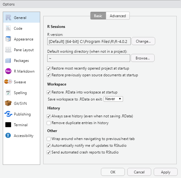
Figure 2.10: The workspace settings can be adjusted in Tools | Global Options.
The section “Save workspace to .Rdata on exit” prompt allows 3 options: “Always”, “Never”, and “Ask”. If you’ve seen this prompt when you exit R, you likely have the “Ask” option set. If you haven’t been seeing this prompt, select the “Ask” option (you can change it back after this chapter). Now, when you exit R, you’ll be asked whether you should save your workspace or not.
Normally, if prompted to save the workspace, you can choose Don’t Save. But let’s just see what happens when you answer that question Save. Make sure the option “Restore .RData into workspace at startup” is also checked.
Exercise:
- Save your file.
- Close out of RStudio, this time when RStudio closes and asks if you’d like to save the workspace image, select “Save”.
- Open your file again.
What happened? As before, your script opens in the script pane.
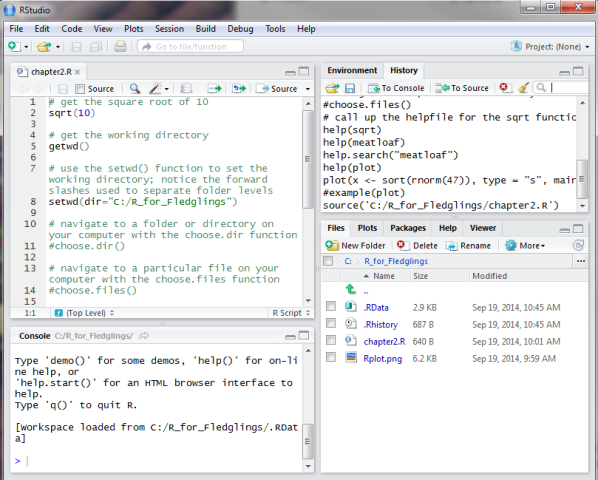
Figure 2.11: The Workspace has been reinstated. The history commands and all objects in the Global Environment were saved in the .RData file.
- Click on the History tab, and you’ll see that all of the commands you entered in the previous session appear.
- Click on the Global Environment tab and you should see that your environment is restored.
- Look in the Files tab, and you should see a new file called .RData. This file stores the workspace information.
- Clear objects from your Global Environment.
- Click on that .RData file, and you’ll be asked whether you want to load the R data (objects) into the global environment.
- If you select Yes, the objects will appear in the Global Environment again.
- Look at your console and note: most of the RStudio button clicks are actually function calls to R.
You may find that you rarely save the workspace if the code can be quickly re-run to generate your objects. In that case, the “Never” option may be right for you. There are times, however, when you will want to save certain elements of the workspace so that you don’t have to re-create the objects. You’ll see how this is done in future chapters.
Some things to note about the Global Environment in RStudio:
- You can clear the environment by clicking on the “clear” button (with the little broom). This works with individually selected items as well.
- You can view the environment in the R console by typing in ls(). This invokes the
lsfunction, which lists all of the objects in the workspace. - You can remove objects from the environment in the R console by using the
rmfunction, which is the “remove” function. This function takes arguments that are environment objects. So rm(x) will remove x from your environment. - You can save the entire environment and history (jointly called the “workspace”) by pressing the save button. Or you can type save.image() in the console, which invokes the
save.imagefunction. - You can save individual items of the workspace with the
savefunction. So save(x) will save individual objects in the workspace. - The
loadfunction can be used to load an object back in.
2.5 R Studio Settings
Now that you have a brief introduction to RStudio’s panes, let’s take a quick look at the program’s options, where you can control settings such as font size, etc. Go to Tools | Global Options, and you should see the following box appear:
Figure 2.12: The ‘General’ tab in the Global Options.
We’ve already touched on the Workspace section in the dialogue box in the “General” tab section. We won’t go through each and every section here, but rather want to just highlight each section and encourage you to become familiar with the options, even if you don’t touch a thing.
Exercise: Click on each section, and explore the various settings available to you.
- General - look but don’t touch until you’ve finished R for Fledglings. Well, OK - you can change the Workspace settings to your desire. Our personal preference is to turn off the “Restore .Data into workspace at startup” and to set the “Save workspace to .RData on exit” to “Never”. We can use R functions to intentionally do these things rather than wonder why they are auto-magically done for us.
- Code editing - make sure the soft wrap option is selected; this will ensure that lines of code are automatically wrapped so you don’t have to press return when you get to the end of a line.
- Appearance - choose a color scheme that works for you. You may also select the Editor font size and zoom level here.
- Pane layout - use the default layout for the duration of this book.
- Packages - make sure “enable packages pane”" is checked. We’ll cover packages in the next chapter.
- Sweave - look but don’t touch.
- Spelling - allows a spell-check of your files.
- Git - options for saving multiple versions of your code, and for working on script files with multiple contributors.
- Publishing - allows you to publish R outputs to the web.
- Terminal - look but don’t touch.
- Accessibility - look but don’t touch (unless needed).
2.6 The R Studio Toolbar
Like most computer programs, RStudio has a toolbar where you can access many commands. We’ll have you briefly peer into each menu item now, but will learn about the various options as we need them in our Tauntaun exercise.
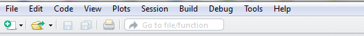
Figure 2.13: Take some time to explore the RStudio toolbar.
Exercise: Click through each of the toolbar menu items, and explore the various options.
- File
- Edit
- Code
- View
- Plots
- Session
- Build
- Debug
- Tools
- Help
The Help menu is of particular importance. It allows you to check for updates and find keyboard shortcuts that save time. It also lets you gain access to all-important documentation. The RStudio documentation is found here, while the RStudio support and tutorials can be found here.
You should see that we’ve already used several of these options by clicking on a button somewhere else in RStudio. Like most programs, there are usually several different ways of achieving the same thing. There’s more than one way to skin a Tauntaun!
2.7 The R Studio Cheatsheet
RStudio conveniently points to printable “cheatsheets” that you find useful. Go to Help | cheatsheets, and there you will find the RStudio IDE Cheat Sheet. Clicking on the link will download the cheatsheet pdf to your system, where you can print or save it for future reference.
2.8 Answers to Chapter 2 Exercises
Exercise:
Below are a few common functions that you might have used in Excel if you are a spreadsheet user. We list the familiar names of the functions Excel uses to take an average (‘average’), compute the standard deviation (‘std’), find a value in a range specified cells (‘index’), calculate the sum (‘sum’) or find the minimum value (‘min’) for a range of cells. R has functions that do these things too, but the names of the functions may be different! Try the help, ?, help.search, and ?? approaches. Failing those, try Google.
- average (a tricky one; this is the arithmetic mean)
- std (another tricky one; this is the standard deviation)
- match
- sum
- min
1.  average - `mean`
2.  std - `sd`
3.  match - `match`
4.  sum - `sum`
5.  min - `min`