10 R Markdown
Packages needed:
 * rgdal - for working with spatial data
 * tidyr - for data wrangling
 * dplyr - for data wrangling
 * knitr - for knitting the Rmarkdown document
 * rcrossref - for creating and rendering a bibliography
Install and load these packages now!
Now that your harvest dataset is cleaned and merged with hunter information, and you have a few plotting, summary, and statistical analysis functions up your sleeve, you’re ready to begin your Tauntaun annual report. This report will summarize the number of animals harvested by town, age, sex, harvest method, and hunter residency, and is submitted to the U.S. Fish and Wildlife Service each year. It must be polished and submitted as a pdf report. Your own agency also wishes to publish this report on its website, and is requesting an HTML file that is easily accessible to web-users. We can do ALL of this through R!
In this chapter, we’ll introduce you to R markdown, an easy-to-write plain text formatter designed to make web content and reports easy to create. Reproducibility is the name of the game, which is defined by Wikipedia as “the ability of an entire experiment or study to be reproduced, either by the researcher or by someone else working independently. It is one of the main principles of the scientific method and relies on ceteris paribus.” In case you were wondering, ceteris paribus means “all other things being equal or held constant”. With R markdown, it is easy to reproduce not only the analysis used, but also the entire report.
The advantage of using R markdown (versus a script) is that you can combine computation with explanation. In other words, you can weave the outputs of your R code, like figures and tables, with text to create a report.
For example, let’s assume you want this text in your Tauntaun annual report:
The total Vermont Tauntaun harvest in XX was XX
We want to replace the blue XX’s with R output. Using R markdown, we insert “secret” R code into the R markdown file that calls in the cleaned harvest dataset, creates objects that identify the year (year.tag <- 1901), subsets the data by the year (harvest <- subset(harvest, year == year.tag)), and sums the harvest (observations <- nrow(harvest)). Then, using R markdown code, we replace the XX’s with our R objects, roughly along the lines of:
The total Vermont Tauntaun harvest in year.tag was observations .
If year.tag = 1901 and observations = 3222, then our final HTML output becomes:
The total Vermont Tauntaun harvest in 1901 was 3222 .
To illustrate these basic concepts, let’s read in our super-cleaned and merged TauntaunData.RDS file and remind ourselves how it is structured:
# read in the Tauntaun dataset
TauntaunData <- readRDS("datasets/TauntaunData.RDS")

# look at its structure
str(TauntaunData)
## 'data.frame': 13352 obs. of 19 variables:
## $ hunter.id : num 560 89 49 108 225 633 146 12 602 462 ...
## $ age : num 1 1 3 3 1 3 1 1 1 4 ...
## $ sex : Factor w/ 2 levels "f","m": 1 1 2 1 2 1 2 1 2 2 ...
## $ individual : num 116 53 822 795 468 809 347 144 384 902 ...
## $ species : chr "Tauntaun" "Tauntaun" "Tauntaun" "Tauntaun" ...
## $ date : Date, format: "1901-10-01" "1901-10-01" "1901-10-01" "1901-10-01" ...
## $ town : Factor w/ 255 levels "ADDISON","ALBANY",..: 1 21 90 93 96 134 146 158 224 8 ...
## $ length : num 294 315 427 270 448 ...
## $ weight : num 677 880 1039 624 1109 ...
## $ method : Factor w/ 3 levels "bow","lightsaber",..: 2 1 3 2 2 1 3 2 2 2 ...
## $ color : Factor w/ 2 levels "White","Gray": 1 2 1 2 1 2 2 2 2 2 ...
## $ fur : Factor w/ 3 levels "Short","Medium",..: 3 3 2 2 3 1 3 1 2 3 ...
## $ month : num 10 10 10 10 10 10 10 10 10 10 ...
## $ year : num 1901 1901 1901 1901 1901 ...
## $ julian : num 274 274 274 274 274 274 274 274 274 275 ...
## $ day.of.season: num 1 1 1 1 1 1 1 1 1 2 ...
## $ sex.hunter : Factor w/ 2 levels "f","m": 2 2 2 2 2 1 2 2 2 2 ...
## $ resident : logi FALSE TRUE TRUE TRUE TRUE TRUE ...
## $ count : num 1 1 1 1 1 1 1 1 1 1 ...Next, let’s enter code to generate a frequency histogram by age when year.tag = 1901:
# create a year.tag object
year.tag <- 1901

# subset the data by the year.tag
data  <- subset(TauntaunData, year == year.tag)

# compute the the total harvest
observations <- nrow(data)

hist(x = data$age,
     breaks = 6,
     xlab = "Age",
     main = paste0("Total Harvest for ", year.tag, "; n = ", observations),
     col = "orange")
Figure 10.1: Tauntaun harvest with year.tag = 1901.
If you change only the year value in your R markdown file (year.tag <- 1902), and then rerun code above, the objects, text, and plot will automatically update:
Figure 10.2: Tauntaun harvest with year.tag = 1902.
How cool is that? By creating your annual report as an R markdown file, you use R to quickly generate “canned” output like tables, figures, etc. This allows you much more time to do important things, like interpret the output and deeply consider its implications.
10.1 HTML Markup vs. Markdown vs. R Markdown
Before launching into R markdown, let’s first touch on what exactly is “HTML”, “markdown”, and “R markdown”.
HTML stands for Hyper Text Markup Language. From w3schools we learn that:
- HTML is a markup language.
- A markup language consists of sets of markup tags.
- The tags describe (format) the document content.
- HTML documents (web pages) contain HTML tags and plain text.
- HTML tags normally come in pairs like <b> and </b>. This is the “bold” tag.
- The first tag in a pair <b> is the start (or opening) tag, the second tag </b> is the end (or closing) tag.
- The end tag is written like the start tag, with a forward slash before the tag name. Everything nestled between these tags will appear in bold font when rendered on a web browser.
- For example, if we want to put the word “Tauntaun”" in bold in an HTML document, we would type this: <b>Tauntaun</b>.
- You’re reading a webpage right now, so let’s look at the HTML code used to display this page. In Edge, right-click on the page and select View source, and you’ll be looking at the HTML code that your browser is interpreting. In Firefox, go to Tools | Web Developer | Inspector. In Chrome, right-click on the page and select View page source. It doesn’t matter what browser you use to peek at the source code. But, holy crow! There are tons of different tags, each doing their own thing. If you are a webpage designer, you know all about tags. For those of us who are not webpage designers, markdown is a great alternative for creating formatted web content.
Markdown is a language designed to make it easy to add formatting to an HTML document, like headers, bold, bulleted lists, and so on. Remember all of those tags you just looked at? We certainly didn’t type those in. Instead, the document you are reading was created with markdown formatting. To bold the word, Tauntaun, we just surrounded the word of interest with sets of double asterisks, which is the markdown syntax for bolding text: **Tauntaun**. A program is then needed to convert the markdown shortcuts into HTML tags. An R package that does this is the package, markdown.
R markdown is a type of script that allows you to combine text that is formatted using markdown shortcuts (like annual report text) and R code (entered in “code-chunks”, which allow you to separate your text from R code). For example, the sentence “The total Vermont Tauntaun harvest in year.tag was observations ” combines text with the R objects, year.tag and observations. R objects can be tables, figures, maps, and pretty much anything in between. Note: the actual syntax for how to insert the R objects will be explained later.
To give you a better idea of how HTML, Markdown, and RMarkdown vary, consider the figure below. We’d like to write code that displays the header, R for Fledglings, followed by a date. In the HTML version, the header is enclosed by the tags, <h1> and </h1>. The date is enclosed in paragraph tags, <p> and </p>. Note that the date is hard-coded. In the Markdown version, the tags are done away with; a single hashtag will format the heading R for Fledglings. The date is hard-coded but not wrapped in paragraph tags. In the RMarkdown version, we use markdown syntax to format the heading, but then make a call to R, and use the date function with no arguments to generate today’s date (which happens to be August 15, 2020). Thus, the date is not hard-coded, and the output will be updated each time you produce the R Markdown document.
Figure 10.3: Comparisons of HTML, Markdown, and R Markdown.
In this chapter, you’ll learn about R markdown as a way to produce high quality documents. This chapter is long and full of screen shots, and as such it is divided into three sections to keep things under control.
1) In the first section, we introduce markdown and see it in action so that you can see where we are headed. This work will be saved in a script called chapter10_markdown_intro.Rmd.
2) In the second section, we will create a new Rmd file called TauntaunReport.Rmd. In this section, we will outline our annual report and will create all of the objects that are needed.
3) The third section will continue building out the TauntaunReport.Rmd script, and will involve actually writing our Tauntaun annual report, weaving together the objects created in section 2 along with text.
Follow along with us! If you get stuck, you can download each of these files from the Fledglings website.
10.2 R Markdown Basics (Section 1)
Open up your Tauntaun project (Tauntaun.Rproj). Creating a new markdown file within this project is as easy as going to File | New File | R Markdown . . .. A new dialogue box appears:
Figure 10.4: New R Markdown file.
In the left menu, you have a few options regarding what type of file to create, a document, presentation (slide show, covered in chapter 14), Shiny (a slick web application that allows users to interact with R with a graphicical user interface (GUI) that can be hosted on the web), or template (a pre-formatted document). We’ll be creating a new document. After filling in the author and title, select what output you are interested in. The default is HTML, which will convert your R markdown file into an HTML file, complete with markup tags. This is the option we will use. Later, we can convert this to PDF or Word.
After you make your selection, fill in the details, and press OK. RStudio will display the new file in your Script pane:
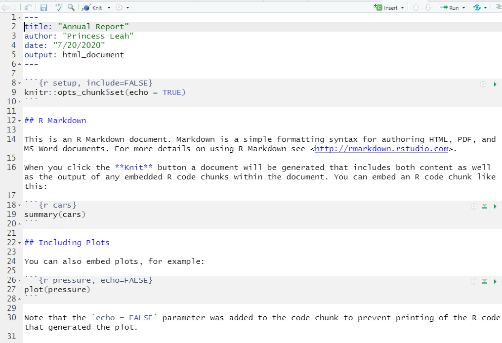
Figure 10.5: A new markdown document.
Save this file now as chapter10_markdown_intro.Rmd.
This is an R markdown document, identified with the .Rmd extension. What you are looking at is an .Rmd template – the developers of RStudio conveniently include a very short R markdown tutorial on the template itself. Notice the information from the previous dialogue box has been neatly inserted into text between sets of three dashes (- - -) (lines 1 and 6). This section is called your “metadata”, and you can modify it as needed (more on this at the end of this chapter).
An R markdown file includes both R code (which are shown in the figure above in gray-shaded sections called “code chunks”) as well as text (which is unshaded). There are three code chunks in this document; each code chunk is contained in a “fence” (the three backticks). The text is formatted with markdown symbols. For example, notice the sentence: “When you click the Knit button….”. Recall that the double asterisks that surround the word “Knit” are markdown syntax. When rendered, the output HTML file will have HTML “bold” tags surrounding the word “Knit”, and this word will appear in bold when viewed in a web browser. RStudio has a markdown syntax cheatsheet, which can be found by going to Help | Markdown Quick Reference Guide. The guide will appear in your Help tab.
Let’s look at a code chunk in more detail. The second code chunk (lines 18-20) is an R code chunk named cars, which invokes R and then uses the summary function to generate a summary for the built-in dataset called “cars”. A bit further down, a third code chunk named pressure uses the plot function to plot the built-in-dataset called “pressure”. See if you can find that. This code chunk has an argument named “echo” which is set to FALSE.
Let’s suppose that this document represents our final report. When you are ready to create your output file (that is, convert your .Rmd file to HTML, PDF, or Word), click on the Knit toolbar button, which is the cool icon with two knitting needles and a ball of yarn. Immediately to the right of the Knit button is a drop-down menu that allows you to select your desired output.
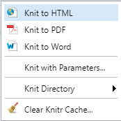
Figure 10.6: Knit options.
Try it now! Knit this sample document, and select the HTML output. Knitter will run each code chunk in order and produce the markdown document, and then convert the markdown to HTML code.
You should see something along these lines:
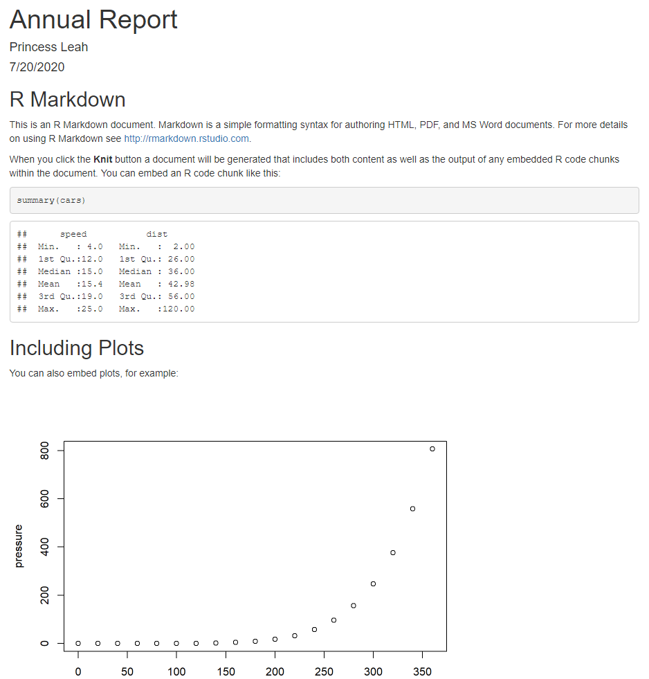
Figure 10.7: Knitted R markdown example.
There are two places that this output can appear. First, it may appear in your Viewer tab in the lower right hand pane of RStudio. Second, it may open a new browser window and display it there. This option may be set by clicking on the gear icon (to the right of the knitting ball):
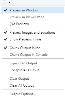
Figure 10.8: R Markdown settings.
The “Knit” button sets several things in motion, and you might have guessed that it executes specific R functions in a specific order. First, it sends your R code chunks to R for evaluation, and formats your output as a markdown file (which has the extension .md). If you select HTML as your output file, it then uses the package markdown to convert the markdown syntax to an HTML document. All of this happens with a single click. If you’re using RStudio, both the markdown and knitr packages are loaded when you create or open an .Rmd file. If not, you’ll want to install and load those packages, and then use the knit function to produce the output.
Let’s look at our HTML document in more detail, and compare it with the .Rmd file. Notice that the metadata was inserted into the top of the new HTML document. The text “This is an R Markdown document….” is displayed. The code chunk that called the summary function is also displayed, along with its output. A bit further down the document, the plot function is used to create a plot, but the R code that produced the plot itself is not displayed. This is because the code chunk option named “echo” was set to FALSE. We’ll discuss these options in more depth below.
Code chunks are fundamental sections of an .Rmd file, so let’s spend a few minutes discussing code chunks.
10.2.1 R Markdown Code Chunks
As we’ve seen, you can’t just start typing R code into the blank .Rmd file. The main difference between an .Rmd file and an .R script file is that any R code is typically inserted as “code chunks”. Let’s see how this works by entering a new code chunk into the R markdown built-in tutorial (the end of the tutorial is just fine).
To insert a new chunk, choose the Insert button, and then select R as shown below, or go to Code | Insert Chunk on the toolbar.
Figure 10.9: Insert a code chunk.
You’ll see that a code chunk has been inserted into your .Rmd file that looks something like this:
```{r }
# enter your code here
```
Notice that the code chunk appears in a different color block in the Editor pane.
Each chunk has the same syntax. The start of the chunk minimally has three back ticks, followed by {r}. The end of the chunk is simply three back-ticks. In between these sections, you enter your R code - whatever code is needed to achieve the results you seek.
There are a few things to point out regarding code chunks. The information about the chunk itself is stored between the curly braces { }. You can enter a name for each code chunk after the letter r followed by a space. This should be something descriptive you come up with to help you remember what the section of code will do, and it is placed in quotes. Then, add any other “chunk” arguments you need, all separated by commas. In RStudio, if you click the “tab” key after the letter r, a pop-up will appear listing the various arguments, and you can tab your way through the options.
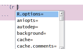
Figure 10.10: Code chunk options are displayed with the help of the tab key.
There are several optional arguments, but the key arguments we’ll discuss for now are:
- echo
- eval
For example, the following code chunk is named “SockChunk”, followed by the arguments “echo” and “eval” and their values. Add this chunk to the bottom of your .Rmd script.
```{r SockChunk, echo = TRUE, eval = TRUE}
socks <- "Darn Tough"
socks
```
The arguments, echo and eval, are logical arguments. Echo = TRUE means “print this R code” when the document is knit. In other words, this code chunk (the actual R code) will be displayed in your report. We saw this option at work in the summary example (code lines 18-20), where both the code and the summary were output upon knitting. Echo = FALSE means that the R code is “secret” and will not appear in the markdown or HTML output. You can still use R objects created by the chunk, but the actual R code that creates them is secret. We saw this option at work in the plot example, where only the plot was output upon knitting (code lines 26-28).
The other argument, eval, indicates whether the chunk should be sent to R for evaluation or not. In report writing, sometimes you create figures or tables that you don’t want to include in the final version. By setting eval to FALSE, you can keep a record of the code used, even if the object doesn’t make the final cut. Additionally, you may have a “problem chunk” where R keeps giving you errors. If future chunks don’t depend on the result from the problem chunk, you can set eval to FALSE, finish the rest of the report, and then return to the problem chunk with a fresh mind. The code in the chunk named SockChunk will be evaluated and displayed when we knit this document because echo = TRUE and eval = TRUE.
As with other functions in R, knit code chunks have default values. The default value for eval is TRUE, and the default value for echo is TRUE. Re-knit your document, and twiddle with the echo and eval settings to see what they do. Remember these are logical arguments, so your options are TRUE or FALSE.
Other code-chunk arguments are also helpful, and we’ll describe what they do when we use them.
To get the most out of markdown, name your chunks well! The names should not have spaces or periods and should be descriptive of the actual code content. By naming the chunks you can quickly find the section of R code of interest (as we’ll see in section 3 of this chapter). However, note that two different code chunks cannot have the same name. You aren’t required to name chunks, and can name only those of particular interest, if desired.
That ends section 1 of this chapter, markdown basics. You can close your file, as we will no longer need it. Hopefully you now know what an .Rmd file is, how it consists of both text and calls to R, and how it “knits” the output. A definitive guide to R Markdown can be found here - we’re just giving you a whirlwhind tour in this chapter by way of introduction.
10.3 Tauntaun Annual Report Outline and R Objects Needed (Section 2)
In this section, we will will create an .Rmd file called TauntaunReport.Rmd. We will outline our Tauntaun annual report, and identify and create the R objects we need for the report – we won’t be weaving R objects with annual report text just yet. These objects will include figures, summary data, tables, etc. To create these objects, we’ll use some old functions that we learned in previous chapters, but also a few new ones. We won’t dwell on the coding details, so make sure to use helpfiles if needed and inspect each line of code. Copying and pasting is no way to learn! Then, in Section 3, we’ll weave in text with these objects. In this way, we can separate the R code explanation from the markdown explanation (with hopefully a more lucid result!).
Open a new .Rmd file and save it as TauntaunReport.Rmd. Delete all of the canned template text except for the metadata. We’ll be adding code chunks to this document one step at a time.
10.3.1 Annual Report Outline
Our first step will be to outline the annual report by paragraph. Let’s do that now, identifying all of the R objects we’ll eventually need to plug into the report. The report will have five main paragraphs (sections), a literature cited section, and an appendix.
- Introduction - basic “canned” text about Tauntauns in Vermont.
- For this section, we’ll need to create an object called year.tag to define the year of interest.
- General Summary for the Year
- For this section, we’ll need to read in the TauntaunData.RDS (the cleaned harvest data merged with the hunter information and spatial information). We’ll then subset this data frame by the year.tag, and will name this subset tauntaun_annual.
- Then we’ll extract summary information, such as total number harvested, largest animal harvested, maximum and minimum harvest.
- Hunter Demographics
- This section will provide information about how many hunters participated in the hunt for our given year, what sex they were, and where they were from (Vermont or out-of-state). We’ll also create a pie chart that presents the total number of harvested Tauntauns by hunting method.
- Analysis of Age and Sex
- This section will summarize the harvest by Tauntaun age and sex. This information will be displayed as a histogram. We’ll use a chi-square test of independence to test if the harvest totals vary by these groups.
- Harvest By Town
- This section will simply indicate the top five towns with the largest harvest, and will re-create the harvest by town map that we did in the last chapter.
- Literature Cited
- What is a report without a citations section? In this section, we will create a .bib file that stores citations that you can use within your report.
- Appendices: Analysis of Harvest by Town
- Tauntaun hunters from a variety of towns in Vermont typically request that your agency provides data on the harvest by age and sex on a town-by-town basis. This section will create a very large table of harvest by town, age, and sex.
As we’ve said, all of the objects will be created ‘chunks’. For each code chunk, we will set the “echo” argument to FALSE so that our code will not appear in the report itself.
10.3.2 Preliminaries
Our first code chunk will simply load all of the R libraries that we’ll need when creating our annual report. This first code chunk will be called “preliminaries”, and we’ll load the packages while suppressing any messages and warnings at start-up. Create a new code chunk from the code below (or use the insert button, and copy the R commands within the code chunk):
```{r preliminaries, echo = F}
# load the required packages for the report
suppressWarnings(suppressMessages(library(tidyr)))
suppressWarnings(suppressMessages(library(dplyr)))
suppressWarnings(suppressMessages(library(rcrossref)))
suppressWarnings(suppressMessages(library(rgdal)))
suppressWarnings(suppressMessages(library(knitr)))
```
A preliminary code chunk is often useful to get some business out of the way. Here, we simply loaded our required packages, but we could set some knitr options here if we wish. Note that if you are using RStudio, you don’t need to install and load the markdown and knitr packages - they are ready to go! Give yourself a line break or two so that you are ready to enter a the next, separate code chunk.
10.3.3 Paragraph 1: Introduction
The introduction of our report will contain basic “canned” text about Tauntauns in Vermont. For this paragraph, we need to create a single object called year.tag. Enter (or copy) the code below into your blank script.
```{r paragraph1, echo = F}
# stores year.tag containing the year of the annual report.
year.tag <- 1901
```
Now execute the code chunk. You can do so by pressing the green arrow in the chunk itself, or going up to the Run button, and choosing Run Current Chunk. You should see that R created the object called year.tag. In your console, type in year.tag and verify that the chunk returned what you were hoping.
## [1] 1901Before moving on, you need to double-check your output. You could enter the code above as a new code chunk, and then set the code chunk arguments eval and echo to FALSE. To check the chunk, press the “Run” button in the chunk itself to run the code (without knitting the document). When you knit your annual report, the chunk that creates the object called year.tag will be run (but not displayed in the output), and the second chunk that tests it will not be evaluated or displayed. Regardless, it is critical that you check your chunk code to make sure it is doing what you intend.
10.3.4 Paragraph 2: General Summary
The next paragraph of our annual report will require a few R objects that contain summary information about the harvest. We’ll need to read in TauntaunData.RDS (the final, super-cleaned data). We’ll then use the subset function to subset TauntaunData by the year_tag. We’ll name this new object tauntaun_annual. Then we’ll extract summary information, such as total number harvested, largest and smallest animals harvested, and dates of the first and last harvest. You’ll see functions such as table, min, max, nrow in use . . . we’ve used these in previous chapters so hopefully they are old-hat by now. Create a new code chunk block, and enter (or copy) the following:
```{r paragraph2, echo = FALSE}

# read in the .RDS file
TauntaunData <- readRDS("datasets/TauntaunData.RDS")

# use the subset function to subset the data by year.tag
tauntaun_annual <- subset(TauntaunData,year == year.tag)

# get the total count
total  <- nrow(tauntaun_annual)

# use the tables function to count the frequency by sex
total.by.sex  <- table(tauntaun_annual$sex)

# get the largest Tauntaun
largest  <- max(tauntaun_annual$length)

# get the smallest Tauntaun
smallest  <- min(tauntaun_annual$length)

# get the first harvest date
first.harvest  <- min(tauntaun_annual$date)

# get the last harvest date
last.harvest  <- max(tauntaun_annual$date)
```
When you run this code chunk, R will create the objects. Once again, it is important to verify that the outputs match what you intend! Let’s check a few in our console (or if you wish, in a new code chunk that duplicates the first, but where ECHO and EVAL are set to FALSE and where the objects the code generates are returned for inspection. Then press the Run button in the chunk itself).
## [1] 931##
## f m
## 490 441## [1] 532.83## [1] 242.32## [1] "1901-10-01"## [1] "1901-12-31"You may have also noticed the tiny arrow heads that appear in your editor’s left hand margin, just to the right of the numbers. Select the down arrow and you can “shrink” or “minimize” your paragraph code blocks. Try it! This helps you to de-clutter your view….you can shrink code blocks you know are working, displaying only the heading as a navigation tool.
At the bottom of your editor pane, look for the symbol  . Yours might say “paragraph 1” or “paragraph 2” instead of “Top Level”. Regardless, click on the little arrows, and you should see the code chunks listed by name. Clicking on an option will bring you to the code chunk.
10.3.5 Paragraph 3: Hunter Demographics
Moving right along, let’s create some objects that will provide information about the hunters themselves. This information will be presented in paragraph 3 of our annual report. In this code block, we’ll create an object (a png file) that will be stored in a new directory called “figures” (a subfolder in your working directory), so you’ll need to create this folder before running the code. Remember that you can create the folder by hand, by clicking on the  icon in the Files tab, or with the
 dir.create function.
Create this folder now!
The code will provide information about how many hunters participated in the hunt, what sex they were, and whether they were Vermont residents or not. Here, we make use of the table function and the prop.table function. We’ll also create a pie chart that depicts the total number of harvested Tauntauns by hunting implement (light saber, bow, or muzzle). Look for the pie function, which will return the pie chart if the chunk is evaluated. We want to store this figure as a png file, so we’ll use the png function to “turn on” a device that can write png files to disk, and then turn the device off.
Note to Mac users: In the
pngfunction call, you may (or may not) need to add the argument named type and set it to “quartz”. Otherwise, the image may not be written to disk.
```{r paragraph 3, echo = F}

# use the table function to generate a table of hunter gender
hunter.gender  <- table(tauntaun_annual$sex.hunter)

# use the table function to generate a table of hunter residency
hunter.residency  <- table(tauntaun_annual$resident)

# use the prop.table function to get the proportions of residents
hunter.residency  <- prop.table(hunter.residency)

# use the table function to get the frequencies of each harvest method
hunter.method  <- table(tauntaun_annual$method)

# run a chi-square analysis to test if the hunter methods are
method.chisq <- chisq.test(hunter.method)

# convert the names to upper case
names(hunter.method)  <- toupper(names(hunter.method))

# build the pie chart labels
lbls <- paste(names(hunter.method), "\n", hunter.method, sep = "")

# create the pie chart; store it as a png file inside the figures folder.
png(filename = "figures/pie.png")

# create the pie chart
pie(hunter.method,
    labels = lbls,
    main = "Total Harvest By Method \n (with sample sizes)",
    sub = paste0("Chi-square = ",
                 round(method.chisq$statistic, 3),
                 " ; p = ",
                 round(method.chisq$p.value, 5)))

# turn the png writer off; prevent messages
invisible(dev.off())
```
Run this chunk, and double check your output either in the console or in a new code chunk dedicated to testing the chunk itself.
Now, take a look in your new folder called figures, and look for the new png file that was created after you ran this code. To get a quick look at the pie chart, re-run the pie function (without turning the png writer on or off) by highlighting the code and pressing Run | Run Selected Lines. You should be able to see the pie chart in the Plots tab of RStudio.
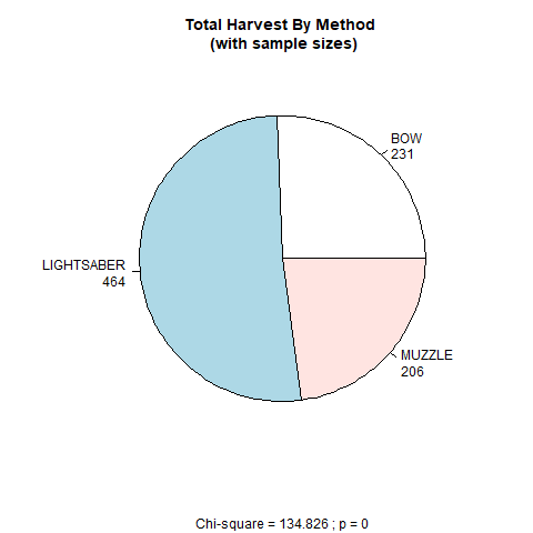
Figure 10.11: Pie chart showing harvest method and Chi-Square analysis.
10.3.6 Paragraph 4: Analysis of Harvested Animals by Tauntaun Age and Sex
The fourth paragraph of our annual report will summarize the harvest by Tauntaun age and sex, and add a few other juicy bits of information pertaining to fur length and color morph. Our first step in the code block will be to add labels to the column, sex, which contains values stored as “m” and “f”. We want these to be displayed as “Male” and “Female” in our report. Then we will use the table function to summarize the data by age and sex, as we have in the past, and run a chi-square test of independence to see if the numbers vary by age and sex categories. We’ll use that same function to tally the numbers by color morph and fur length.
Finally, we will use the barplot function to create a stacked column histogram showing the total harvest by age and sex. Barplot is a very useful function for creating bar graphs. Take a look at the helpfile for barplot, and you’ll see several arguments and examples. You will use a few arguments all of the time, including main (title), col (colors), xlab (x axis label), and ylab (y axis label). This function requires that we transpose our age.by.sex object, which we’ll do with the transpose function, t. This is done so that the ages occupy the x-axis on our plot (instead of sex).
Copy this code into your script, review it, and execute it.
```{r paragraph4, echo = F}

# use the table function to summarize the data by age and sex
age.by.sex <- table(tauntaun_annual[,'age'], tauntaun_annual[,'sex'])

# run the chi-square test
age.sex.chisq <- chisq.test(age.by.sex)

# generate tables of fur color by sex
fur.by.sex <- table(tauntaun_annual$sex, tauntaun_annual$fur)

# generate tables of color by fur
color.by.sex  <- table(tauntaun_annual$sex, tauntaun_annual$color)

# create a barplot of the transposed data in table, age.by.sex.
# store this as a new png file in your new figures folder

png(filename = "figures/age.by.sex.png")
bp <- barplot(t(x = age.by.sex),
              main = paste("Tauntaun Harvest By Age and Sex:", year.tag),
              xlab = "Age",
              ylab = "Frequency",
              col = c("blue","yellow"))

# add the chi-square statistic below the plot title
mtext(text = paste0("Chi-square = ",
                    round(age.sex.chisq$statistic, 3),
                    " ; p = ",
                    round(age.sex.chisq$p.value, 5)),
      side = 3)

# add the legend
legend(legend = colnames(age.by.sex), x = "topright", fill = c("blue", "yellow"))

# put a box around the chart
box()

# turn the png writer off
invisible(dev.off())
```
Once again, make sure to look for these new objects in your global environment and check them! Please don’t just copy and paste this code - make sure you understand each line!
Once again, look for the png file in your figures folder. Once you find the file, click on it to make sure it looks like you want it to:
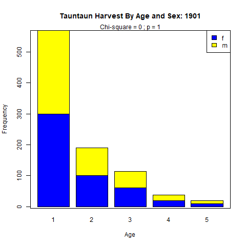
Figure 10.12: Barplot showing frequency of harvest by sex.
Looks great! Of course, you may disagree, and are free to change the argument values and even add more arguments. Experiment with different arguments in barplot until the histogram is just as you like it. Several new arguments may also come in handy, like horiz, which will determine if the bar plot is vertical (horiz = FALSE) or horizonal (horiz = TRUE), and beside, which determines whether the barplot is stacked (beside = FALSE) or grouped horizontally (beside = TRUE). Don’t forget that you can use the colors function (with no arguments) to see a list of all color options in R.
10.3.7 Paragraph 5: Harvest By Town
The fifth paragraph of our annual report will graphically summarize the harvest by town and will identify the town with the most Tauntauns harvested. We will use the package rgdal to create this map, just as we did in previous chapters. The code will basically mimic our previous efforts, so we won’t explain it in detail. In addition to this map, we’ll rank the towns of Vermont in terms of harvested Tauntauns.
First, we’ll use the aggregate function to tally the harvest by town, and then use the rank function to rank the towns. With this function, the highest rank represents the town with the greatest number of harvested animals. Make sure to read the helpfiles and run some examples! The argument x is a vector full of elements to be ranked. The argument na.last has a default of TRUE. This argument indicates how to handle NA’s within the vector to be ranked. The argument ties.method indicates how you’d like to handle ties. For instance, if two towns both have 10 harvested Tauntauns, how should they be reported? Here, we’ll set this option to random, indicating the R will randomly assign ranks for the ties. The numbers are ranked from lowest to highest (with the town harvesting the most animals having the largest rank). If you wish to reverse the order, just negate the vector to be ranked. After the ranks are obtained, we’ll use the max function to find to identify the top 5 towns.
```{r paragraph5, echo = FALSE}

# read in the town shape file that is stored within the towns directory
town.sh <- rgdal::readOGR(dsn = "towns", layer = "VT_Data_-_Town_Boundaries", verbose = FALSE)

# use the aggregate function to sum the total harvest by town
total.harvest <- aggregate(tauntaun_annual$count,
                           by = list(tauntaun_annual$town),
                           FUN = sum)

# rename the columns of total.harvest
names(total.harvest) <- c("TOWNNAME", "Tauntauns")

# merge the total.harvest into the shapefiles attribute table
town.sh <- sp::merge(town.sh, total.harvest,
                      by = 'TOWNNAME',
                      all.x = TRUE)

# replace NA's with 0 (for towns with 0 harvest)
indices <- is.na(town.sh@data$Tauntauns)
town.sh@data[indices, 'Tauntauns'] <- 0

# make the attribute table's row names the town names (for plotting)
row.names(town.sh@data) <- town.sh@data[,"TOWNNAME"]

# use the function spplot to create the map
twn <- sp::spplot(obj = town.sh,
              zcol = "Tauntauns",
              main = paste('Total Harvest By Town: ', year.tag, sep = " "),
              cuts = 5)

# rank the towns by harvest numbers; note the - sign puts
rank.harvest <- rank(-total.harvest$Tauntauns, ties.method = "first")

# store the top five (best) ranks
top.town  <- total.harvest[which(rank.harvest <= 5), 1]
```
After running this code chunk, you should see the outputs in your global environment.
Are you getting an error with this code? If so, make sure your dsn argument is correctly specified in the
readOGRfunction. Mac users in particular should pay attention to this, as the shapefile itself may be nested within another folder called VT_Data_-Town_Boundaries-shp. If so, the correct dsn might be something like dsn = "Tauntauns/towns/VT_Data-_Town_Boundaries-shp".
Here, we do not need to create a png file because we can store the entire map as an object in R called twn. But, we should check our plot regardless in our console:
This ends our the creation of objects needed for the body of the annual report, but we still need to create objects for the literature citation section and the appendix.
10.3.8 Literature Cited
The next section of the annual report will be the Works Cited section. We’ll take a bit of time now to learn about bibliographies in R. There are many options, but here we will focus on a bibtex bibliography and how to create it in RStudio.
The bibiliography management system for markdown is adapted from LaTeX, and is called BibTeX.
A BibTeX reference file is just a text file, and a single reference looks something like this:
@Article{Brown14,
  author =       "Michelle L. Brown and Therese M. Donovan and W. Scott Schwenk
                 and David M. Theobald",
  title =        "Predicting impacts of future human population growth and
                 development on occupancy rates of forest-dependent birds",
  journal =      "Biological Conservation",
  volume =       "170",
  pages =        "311--320",
  doi =          "10.1016/j.biocon.2013.07.039",
  xurl =         "http://www.sciencedirect.com/science/article/pii/S0006320713002711",
  year =         "2014",
  type =         "Journal Article",
}
Each field (author, title, journal, etc.) is called a bibentry. Citations are represented differently depending on whether it is a book, journal article, technical report, book chapter, etc. The first line @Article{Brown14, indicates that this is a journal article entry in your bibliography, and the shortcut (formally called a ‘citekey’ or ‘bibkey’) is called Brown14. The fields are pretty self-explanatory, but two need a bit of explanation:
doi - According to APA, a digital object identifier (DOI) is “a unique alphanumeric string assigned by a registration agency (the International DOI Foundation) to identify content and provide a persistent link to its location on the Internet. The publisher assigns a DOI when your article is published and made available electronically. All DOI numbers begin with a 10 and contain a prefix and a suffix separated by a slash. The prefix is a unique number of four or more digits assigned to organizations; the suffix is assigned by the publisher and was designed to be flexible with publisher identification standards.”
xurl - This field in normally called url, but we’ve changed it (added an x) so that the url does not appear in the printed bibliography. (If the url field is present, it will appear in the citation.)
You can learn more BibTeX formatting here.
The formatting of a BibTex file is so specific that you really don’t want to create one manually. Wouldn’t that be a pain? So what are your options?
First, you can use some of rcrossref’s functions to create your library. These functions can create a bibliography on-the-fly, without having to use a library that is stored on your computer. Let’s load this package now:
Second, if you use a program like EndNote or the free reference manager, Mendeley, your library can be exported in bibTex format, so you can keep using either of these programs as your reference management tool, and then export the library when needed. These programs are very popular because you can import citations from the web from places like Google Scholar or Web of Science. We’ll show you how to export entries from these programs in BibTeX format in a few minutes.
We will include 4 bibliographic entries into our Tauntaun annual report:
- Darth Vulcan? In support of Anakin Skywalker suffering from borderline personality disorder.
- Han Solo vs. Luke Skywalker on Objectivity, Naturalism, and Publicity
- R
- The R package, rgdal
Two of these entries are journal articles, and of course we need to cite R and the R package, rgdal. We’d also love to include two important blog entries: Science Proves Luke Skywalker Should Have Died in the Tauntaun’s Belly and Inside the Battle of Hoth, but since we don’t know how to cite blogs, we’ll skip it!
10.3.8.1 Creating a Bibliography with rcrossref
With the rcrossref package, you can create references and a literature citation section on-the-fly. In the background, rcrossref calls CrossRef to locate the citation’s metadata. Click here to see exactly where R is sending your query. Do this now!
The rcrossref package allows you to search CrossRef in many different ways, such as by funder, dates, license information, or journal. The function we’ll use next is called cr_works, which searches CrossRef works (articles). Let’s look at the help page:
If you’ve read the help page, you’ll know there are many ways to find what you are looking for. You can search by DOI number or by query, and you can further limit the search results, sort them, and select exactly what you want returned. Let’s try finding the citation for the article, “Is Anakin Skywalker suffering from borderline personality disorder”:
## $meta
##   total_results                                                       search_terms start_index items_per_page
## 1       5708875 Is Anakin Skywalker suffering from borderline personality disorder           0              1
##
## $data
## # A tibble: 1 x 27
##   alternative.id container.title created deposited published.print doi   indexed issn  issue issued member page  prefix publisher reference.count
##   <chr>          <chr>           <chr>   <chr>     <chr>           <chr> <chr>   <chr> <chr> <chr>  <chr>  <chr> <chr>  <chr>     <chr>
## 1 S016517811500~ Psychiatry Res~ 2015-0~ 2018-09-~ 2015-09         10.1~ 2020-0~ 0165~ 1-2   2015-~ 78     625-~ 10.10~ Elsevier~ 5
## # ... with 12 more variables: score <chr>, source <chr>, title <chr>, type <chr>, update.policy <chr>, url <chr>, volume <chr>, assertion <list>,
## #   author <list>, link <list>, license <list>, reference <list>
##
## $facets
## NULL
There’s quite a bit of information in this reference. You can see the authors, title, journal, volume, and even the web address. Once you are sure this is the article you seek, you can create the BibText entry with the cr_cn function (CrossRef citation) by passing in the doi number, and specifying ‘bibentry’ for the format argument:
## $doi
## [1] "10.1016/j.psychres.2015.07.039"
##
## $url
## [1] "https://doi.org/10.1016%2Fj.psychres.2015.07.039"
##
## $year
## [1] "2015"
##
## $month
## [1] "sep"
##
## $publisher
## [1] "Elsevier {BV}"
##
## $volume
## [1] "229"
##
## $number
## [1] "1-2"
##
## $pages
## [1] "625--626"
##
## $author
## [1] "Anthony Tobia and Thomas Draschil and Aphrodite Zimmerman and Jason Breig and Stephanie Peters and Derek Rudge and Danielle Velez"
##
## $title
## [1] "Darth Vulcan? In support of Anakin Skywalker suffering from borderline personality disorder"
##
## $journal
## [1] "Psychiatry Research"
##
## $key
## [1] "Tobia_2015"
##
## $entry
## [1] "article"
This is very useful information, and we would like to store it as a Bibtext entry (along with the other references we need) in a text file so that it can be used in our Tauntaun annual report. Luckily, there is an easy way to do this:
On installation of rcrossref you get an RStudio Addin. To use the Addin, we need to create a shortkey key to use the addin. Then, when you use the shortcut keystrokes, a GUI will open where you can enter and retrieve information from CrossRef. Further, if citations are found, you can add the citation to a file called crossref.bib.
Let’s take time to do this now. Go to Tools | Addins, and you should be greeted with a dialogue box like this:
Figure 10.13: A list of add-ins.
You can see many add-ins that you probably didn’t know existed! You should be able to find the rcrossref add-in by typing its name in the filter box:
Figure 10.14: Find the rcrossref package.
Now that we know crossref exists as an RStudio add-on, we need to assign a shortcut to launch it. You can access the keyboard shortcuts by clicking Tools -> Modify Keyboard Shortcuts…. Then filter to the crossref name as shown below. Here, you will click in the column labeled “Shortcut” and type in your desired shortcut. You can choose any shortcut you want, but beware of overwriting existing shortcuts (which can be found under Tools | Keyboard Shortcut help). We’ve selected Ctrl+Alt+R. RStudio’s help page calls this “binding” the shortcut to a command.
Figure 10.15: Add a shortcut for creating a crossref reference.
You can modify a command’s shortcut by clicking on the cell containing the current shortcut key sequence, and typing the new sequence you’d like to bind the command to. As you type, the current row will be marked to show that the binding has been updated, and the shortcut field will be updated based on the keys entered.
Once you are happy with your selection, press the “Apply” button.
Now that we have a shortcut, let’s use it. Place your cursor in the Rmd file (outside of a code chunk, that is) and press your shortcut strokes. You should be greeted with a friendly dialogue box that allows you to work with Crossref more directly. This is actually a “Shiny” application - a “web-like” application that allows users to interact with R via a GUI instead of the console. While this application is open, R will be “listening” for your inputs into this dialogue box (and will not be available for working in R until you press either the “Cancel” or “Done” buttons at the top of the GUI).
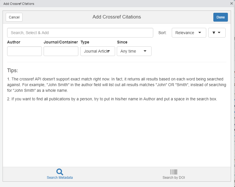
Figure 10.16: Typing the shortcut will bring up a Shiny Crossref app.
The Shiny app is pretty straight-forward: you enter a search string, and almost immediately a call to the Crossref is made, returning potential hits.
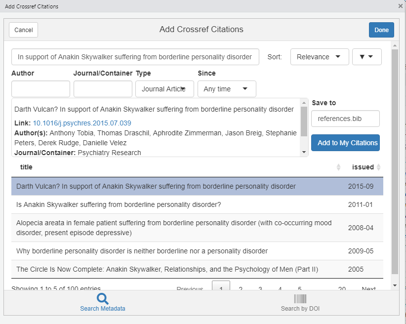
Figure 10.17: Typing the shortcut will bring up a Shiny Crossref app.
Select the reference of interest, then press “Add to My Citations”. Notice that the citations are being stored in a file called references.bib. Wait until you receive confirmation that it has been added. Then press “Done”.
Let’s use our shortcut again to call up the Crossref Shiny app, and try to locate “Han Solo vs. Luke Skywalker on Objectivity, Naturalism, and Publicity”:
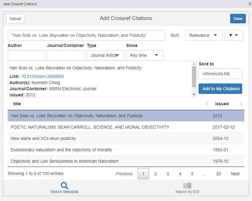
Figure 10.18: Typing the shortcut will bring up a Shiny Crossref app.
Once again, select the reference of interest, then press “Add to My Citations” and await confirmation that it has been added. Then press the “Done” button.
Now, let’s have a look at the file, references.bib. You should see this in your working directory (in the Files tab). Open it up, and have a look! You can add as many references to this file as you’d like . . . it’s just a text file full of biobliographic entries, formatted in a specific way.
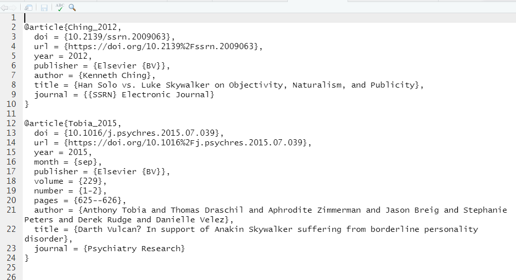
Figure 10.19: Your references.bib file should have two references.
Although the .bib file needs to contain the entries that will be included in your report, it can hold an unlimited number of entries (including those not used in your report).
We have two more citations to add, and here we will make use of the citation function. First, let’s create the citation for R:
##
## To cite R in publications use:
##
##   R Core Team (2020). R: A language and environment for statistical computing. R Foundation for Statistical Computing, Vienna,
##   Austria. URL https://www.R-project.org/.
##
## A BibTeX entry for LaTeX users is
##
##   @Manual{,
##     title = {R: A Language and Environment for Statistical Computing},
##     author = {{R Core Team}},
##     organization = {R Foundation for Statistical Computing},
##     address = {Vienna, Austria},
##     year = {2020},
##     url = {https://www.R-project.org/},
##   }
##
## We have invested a lot of time and effort in creating R, please cite it when using it for data analysis. See also
## 'citation("pkgname")' for citing R packages.
Here, we can copy the section for the BibTex entry (beginning with @Manual and including the curly braces and everything in between), and paste this entry into the references.bib file. Next, let’s get the citation for the package, rgdal:
##
## To cite package 'rgdal' in publications use:
##
##   Roger Bivand, Tim Keitt and Barry Rowlingson (2020). rgdal: Bindings for the 'Geospatial' Data Abstraction Library. R package
##   version 1.5-16. https://CRAN.R-project.org/package=rgdal
##
## A BibTeX entry for LaTeX users is
##
##   @Manual{,
##     title = {rgdal: Bindings for the 'Geospatial' Data Abstraction Library},
##     author = {Roger Bivand and Tim Keitt and Barry Rowlingson},
##     year = {2020},
##     note = {R package version 1.5-16},
##     url = {https://CRAN.R-project.org/package=rgdal},
##   }
Now your references.bib file should look something like this:
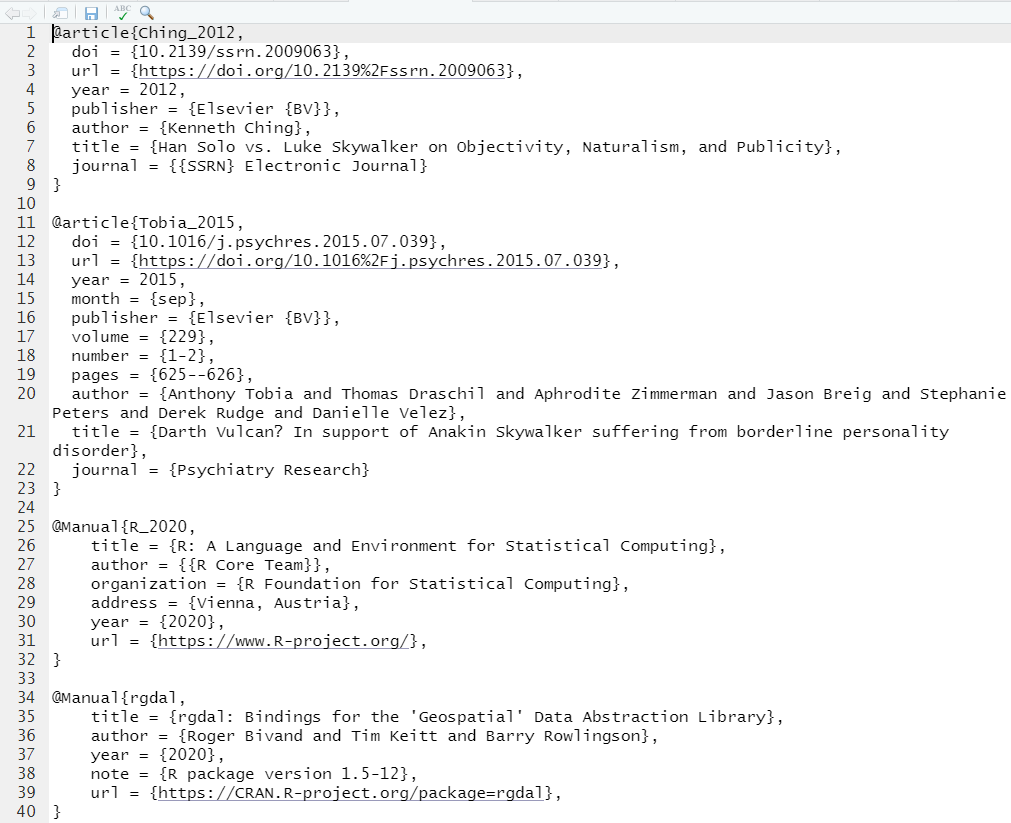
Figure 10.20: Your references.bib file should contain 4 references.
You will want to add a “citekey” for the two references that were just added. For examples, look at the citekeys called Ching_2012 and Tobia_2015 in our first two references. You can find these immediately after the opening curly brace. We added R_2020 and rgdal as citekeys for the last two references. We’ll need these citekeys for our annual report.
Bibliographic management is a critical task for any scholar, and many people use dedicated biobliography management programs for organizing citations, such as EndNote or Mendeley. If you use these programs, and like how they perform, there is absolutely no reason why you can’t keep using them. Let’s have a look at how you can create a .bib file if you use Endnote.
10.3.9 Creating a Bibliography with Endnote
If you use EndNote, you can easily export a .bib file with 5 easy steps:
- Open EndNote library and open the reference list.
- Select the citations to be exported. You can do this by selecting them individually, or create a group.
- Go to File | Export. Make sure that the output style is BibTeX Export. Then name the file to be exported something like biblio.txt, and export it to your Tauntaun project folder. This will be a text file, and you can change its extension to .bib later.
- Open your file up with a text editor, like Notepad++ or RStudio.
- Look at your citations. If you’d like, add citation shortcuts (cite keys) for your entries. Every reference begins with @article{ Immediately after the curly brace, you’ll want to add in a unique ‘citekey’, followed by a comma. While there is no actual convention, informally the convention is the author’s last name, followed by the year such as @Article{Brown14,. These cite keys can be used as shortcuts when using
citeporcitetin markdown.
Now we can move on to the final section of the report, the Appendix, and store it as an object.
10.3.10 Report Appendix
Tauntaun hunters from a variety of towns in Vermont often request that your agency report on the harvest by age, sex, and town. This last code block will be named appendix, and it will create a large table of harvest by town, sex, and age.
To create the data, we’ll first summarize the harvest data with dplyr functions, grouping by town, sex, and age. Then, we’ll convert the resulting dataframe from “long” format to “wide” format with the spread function in the tidry package. This package has many useful functions for working with data, and we encourage you to explore it. Here’s our last code chunk; it will create an object called town.summary.table.
```{r appendix, echo = F}
town.summary.table <- tauntaun_annual %>%
group_by(town, sex, age) %>%
summarise(n = sum(count)) %>%
spread(age, n, fill = 0)
```
We could take time to spruce up this table a bit more, but we’ll press on. Let’s peek at this object to see what it will look like when the document knits. You’ll see that it is a tibble:
## # A tibble: 419 x 7
## # Groups:   town, sex [419]
##    town      sex     `1`   `2`   `3`   `4`   `5`
##    <fct>     <fct> <dbl> <dbl> <dbl> <dbl> <dbl>
##  1 ADDISON   f         1     0     0     0     0
##  2 ADDISON   m         1     1     0     0     0
##  3 ALBANY    f         1     2     2     0     0
##  4 ALBANY    m         2     0     0     0     0
##  5 ALBURGH   f         0     1     0     0     1
##  6 ALBURGH   m         1     1     0     0     1
##  7 ANDOVER   f         3     0     0     0     0
##  8 ANDOVER   m         0     0     3     0     0
##  9 ARLINGTON f         1     1     0     0     0
## 10 ARLINGTON m         0     0     1     1     0
## # ... with 409 more rows
We’ve finished creating the objects we need for our report. To summarize this section, we have an object called year_tag which we can use to pull out harvest data for any given year. For a given year, we also have several objects that summarize the harvest, and two png files that present our results graphically. We also have a slick town map, a bibliography called references.bib, and a detailed appendix.
We’ve finished section 2 of this chapter. Save this file now before you continue.

Figure 10.21: Take a break!
10.4 Weaving Markdown with R (Section 3)
10.4.1 Markdown Syntax
At last we are ready to start with the report text. All of the objects we need have been created in the previous code chunks. All of the code chunks above will be evaluated, creating the objects we need to combine with text. Now it is a matter of writing the report, creating some “canned” text, and filling in sections of the report by calling the objects we have created. This should go quickly and involves more copying and pasting.
Our first step will be to add a line to your metadata that points to your references.bib file.
---
title: "Tauntaun Annual Report"
author: "Princess Leah"
date: "Saturday, August 15, 2020"
output: html_document
bibliography: references.bib
---
We’ll be using markdown syntax to format our report, so before we get started entering text, let’s take a brief look at what these markdown shortcuts are.
-To create a header, precede your text by #. The number of # will determine how large the header is and it will be automatically bold.
-To create italics, surround your text with one set of asterisks (e.g., *italics*).
-To create bold font, surround your text with two sets of asterisks (e.g., **bold**).
There are many more markdown shortcuts, and you can find them by going to Help | Markdown Quick Reference.
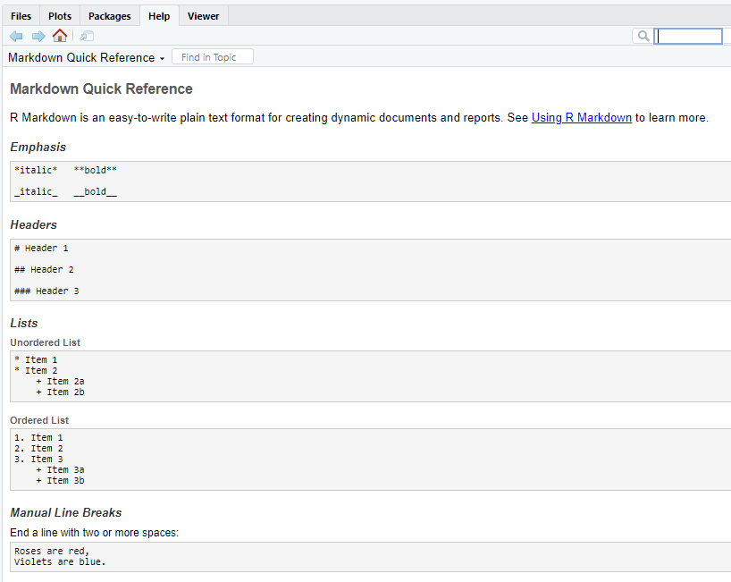
Figure 10.22: Mardown Quick Reference Guide.
Take a few minutes to review this material before pressing on. This quick reference provides almost all of the information you will need to format your annual report.
10.5 The Tauntaun Annual Report
At long last we are ready to start writing our report in markdown. We’ll provide the necessary text and associated code chunks, and will follow along with the outline we set up earlier:
- Introduction - basic “canned” text about tauntauns in Vermont.
- For this section, use the object called year_tag to define the year of interest.
- General Summary for the Year
- For this section, we’ll call up some of the summary statistics we created, such as total number harvested, largest animal harvested, maximum and minimum harvest. We will insert this summary information into a general summary paragraph in our report, as we showed in our example.
- Hunter Demographics
- This section will provide information about how many hunters participated in the hunt, what sex they were, and where they were from (Vermont or out-of-state). Here, we’ll insert our pie chart (png file) that presents the total number of harvested tauntauns by hunting method.
- Analysis of Age and Sex
- This section will summarize the harvest by tauntaun age and sex, displayed as a histogram and saved as a png file.
- Harvest By Town
- This section will call in the R object called twn.
- Literature Cited
- This section will include our literature cited.
- Appendices: Analysis of Harvest by Town and County
- This section will call in the R object called town.summary.table.
10.5.1 Paragraph 1: Introduction
In your R markdown script pane, type a brief introduction (copy and paste the following code, but make sure to not include our hard returns, which we added strictly for the book presentation. However, do make sure to leave at least one blank line before and after each markdown header.
### Introduction

Tauntauns are omnivorous reptomammals indigenous to the icy planet of Hoth [see @Ching_2012].
Tauntauns were first observed in the USA in the late 1850's and they have dispersed to most of
the cold-winter states. Han Solo and Luke Skywalker discovered that freshly killed Tauntauns can
sustain human life on Hoth while they were evading capture by the Evil Darth Vadar [@Tobia_2015].
The Department has been tracking the population of Vermont's tauntaun through harvest records
since 1900. The following report summarizes the annual harvest for tauntauns in
 `r year.tag` . All analyses were conducted using the statistical software program,
R [@R_2020].
Though we don’t show it here, if you’d like the word “Introduction” to be different font size, just use markdown syntax and add one, two, or three hashtags before the word (with one hashtag resulting in the largest font.)
Notice how we inserted three citations within this paragraph, as well as the year.tag object. The three citations were added by referencing the citation’s bibkey in square brackets, such as [@R_2020]. There are several options for including citations within your text; click here for more details.
The year.tag object was inserted with the code r year.tag . This is not a chunk, per se, but is an in-line call to R. The results are inserted and maintain the flow of your text. To insert an R call in-line, enter a back tick, followed by the letter r and a space, followed by your R code, followed by another back-tick. With in-line calls, the R code is generally very succinct. In the year.tag example, we used in-line coding to display the year (an object).
Knit this document now to see how things are going. Try to match up the calls to R with the written text.
10.5.2 Paragraph 2: Tauntaun Data Summary
In your Tauntaun report R markdown file, type a couple summary sentences about the annual tauntaun harvest and hunter population. Find the statistics you need for your report in the Environment tab. You should see them there:
- total - the total number harvested
- total.by.sex - the totals by sex
- largest - the longest tauntaun harvested
- smallest - the shorted tauntaun harvested
- first.harvest - the date of the first reported harvest
- last.harvest - the date of the last reported harvest
Copy the following into your .Rmd file. Again, make sure to delete our hard returns, which we added strictly for the book presentation. Also importantly, make sure to add a return or two after your paragraph headings.
### Summary

Vermont's  `r year.tag`  Tauntaun season resulted in a total harvest of
 `r total`  Tauntauns. Of these,  `r total.by.sex['f']`  were females
and  `r total.by.sex['m']`  were males.  The first Tauntaun was harvested on
 `r first.harvest` , and last Tauntaun was harvested on
 `r last.harvest` .  The range in Tauntauns was characteristic of the population,
ranging from  `r smallest`  to  `r largest`  meters.
Knit this document now to see how things are going.
Now we’re rolling! Notice the code r total.by.sex['f'] . Here, we use in-line R coding, and reference the object called total.by.sex (a table) and extract the element named “f”. In-line coding can be more extensive, but generally long code is written in chunks to return the object you need, and then called in-line.
10.5.3 Paragraph 3: Hunter Summary
Our next paragraph can be quite short, referencing the number of hunters by sex and by residency. In this paragraph, we will also add in our pie chart of harvest method. Recall, the pie chart is stored in the figures folder in your working directory. The objects created for this section include:
- hunter.gender (a table)
- hunter.residency (a table)
- pie (a figure stored in our figures directory)
Copy the following code into your .Rmd file.
### Hunter Statistics
Vermont is well known for attracting hunters of all ages and both sexes. A total of
`r length(unique(tauntaun_annual$hunter.id))` hunters reported a harvested animal, of which
`r hunter.gender['f']` were female and `r hunter.gender['m']` were male.
Resident Vermonters comprised `r paste(round(hunter.residency['TRUE'],2) * 100,'%',
sep='')` of the total hunter population. The harvest method of choice is shown in the
pie chart below.
The very last code is the markdown syntax for inserting figures. Make sure to read the markdown helpfiles. In between the brackets, you can add a figure caption, such as Figure 1. In between the parentheses, you should recognize a file path to your figures folder, and then to the pie.png file that was created in a previous code chunk.
Another option exists for adding figures, and that is through a dedicated code chunk, like this.
```{r, echo = F, fig.cap = "Figure 1."}
knitr::include_graphics('figures/pie.png')
```
This approach uses the include_graphics function from knit (this is the approach we have been using to write this book). Chose either of these approaches (but not both) to display Figure 1 in your report. If you include both methods, the pie chart will appear twice in your report!
When you knit your .Rmd file, your pie chart should be inserted. Try knitting your document now!
10.5.4 Paragraph 4: Analysis of Age and Sex
The next paragraph of your report will describe the age and sex of Tauntauns, and will call in your histogram. Add the following code to your R markdown file, removing any hard returns:
### Analysis by Age and Sex
Vermont's `r year.tag` Tauntaun season resulted in `r colSums(age.by.sex)['f']`
female harvests and `r colSums(age.by.sex)['m']` male harvests. Of the males,
`r fur.by.sex['m', 'Long']` had long fur, while
`r fur.by.sex['m', 'Short']` had short fur. Traditionally, hunters have targeted
the long-fur Tauntauns for their extra warmth. Of the total females,
`r color.by.sex['f', 'White']` were white in color. This color morph
in females has been increasing over time. The harvest varied by age group as well,
as shown in the graphic.

When you knit your .Rmd file, your bar plot should be inserted. Knit your document now!
10.5.5 Paragraph 5: Harvest by Town
The next paragraph will describe the harvest by town, with the main result being the map that was produced. For this, we need a simple call to R that runs the print function. Copy the code below into your .Rmd script (removing hard returns of course)
### Analysis By Town

Harvest was summarized by town with the R package, rgdal [@rgdal].   The town of
 `r top.town`  harvested the most animals.  The full representation of the
harvest by town is shown below.
At this point, you should add the following code chunk:
```{r town, echo = FALSE}
print(twn)
```
10.5.6 Bibliography
The last section of your report will include a citations section. Here, you’ll type in the following:
### Bibliography
Now for the bibliography. Enter the following code after your header. It should NOT be included within an R code chunk as it is really HTML code.
<div id = "refs"></div>By default, knitr will add your bibliography to the end of your document. However, you can add it where you wish by entering a “div” tag, as shown above. Knit once more to check your work! If by chance you don’t see the bibliography, make sure that your yaml header at the top of your markdown includes bibliography: references.bib.
10.5.7 Appendix
At long last, our report will end with a large table that reports the males and females by age class and by town. We’ve already created the table, so all we have left to do is print it. Here, in your markdown code, simply enter “Appendix” as text (preceding it with the desired number of hashtags), and then use an R code chunk to print the town.summary.table object using the kable function in the package knitr. For chunk options, make sure to set echo to FALSE (or your see a lot of html code) and comment = NA to make your table look nice and clean.
### Appendix
Now add one final code chunk, and we’re done!
```{r appendix, echo = FALSE,  comment = NA}
knitr::kable(town.summary.table)
```
Here, we use the kable function from knitr to print our table. Knit your report now!
10.6 The Annual Report
Well? How does it look? You can navigate between code chunks by clicking on the arrows at the bottom left corner of your script pane. If for some reason you are stuck, you can use our example file on the Fledglings website.
Here’s the beauty of R markdown:
Your report and all of the R code used in data analysis are woven together. You can re-create this entire report and analysis in a snap.
If your annual report uses the same format year after year, you can produce a new report for any year by just changing the year.tag. This may take about 5 seconds. While it may require some initial overhead to prepare the .Rmd file and all of the associated R code to generate R objects, think of how many hours can be saved in the long-run.
This report can export as HTML, PDF, or Word. Even if your annual report is not 100% “canned”, creating an .Rmd file can be a terrific first step for compiling a report. Just export to Word and then “add value.” Instead of spending time creating graphs and tables, now you can spend your time making connections back to the real world of Tauntaun management.
10.7 Controlling the Output and Metadata
As briefly mentioned earlier, you can output your .Rmd file as a PDF or Word document (in additional to an HTML). Click on the down arrow next to the Knit button to access alternative knitting options.
To fully implement those options, you need to know about a few other editing tools you can set to control the output and metadata for .Rmd files. Click the wheel to the right of the knitting ball  and examine your editing options.
There are also options for displaying figures, the table of contents, and setting themes. It is very easy to re-knit and see what the various options do. Make sure to look at changes made to your meta-data in response to your selections.
If you plan to knit to Word or PDF, you will need to install a few programs on your computer.
10.8 Summary
That ends our quick look at R markdown. We’re sure you’ll agree that this is a very powerful way to create reproducible reports. And we have only scratched the surface with respect to the kinds of summaries and objects that can be included. We owe a great deal of debt to the developers of R, R markdown, and RStudio.