
Treatment of Missing Data--Part 1
David C. Howell

Missing data are a part of almost all research, and we all
have to decide how to deal with it from time to time. There are a
number of alternative ways of dealing with missing data, and this
document is an attempt to outline those approaches. The original
version of this document spent considerable space on using dummy
variables to code for missing observations. That idea was
popularized in the behavioral sciences by Cohen and Cohen (1983).
However, that approach does not produce unbiased parameter
estimates (Jones, 1996), and is no longer to be
recommended--especially in light of the availability of excellent
software to handle other approaches. For a very thorough
book-length treatment of the issue of missing data, I recommend
Little and Rubin (1987) . A shorter treatment can be found in Allison (2002) . Perhaps the nicest treatment of modern approaches can be found in Baraldi & Enders (2010).
A chapter that I wrote on missing data (Howell (2007) can be downloaded at Missing Data File
I am in the process of revising
this page by breaking it into at least two pages. It has grown much too long and probably no one is eager to
read all the way through it. When I am done, this page will cover missing data in general and focus primarily on the situation where we either look for ways to use the data in its original form, or use traditional missing data techniques such as listwise deletion and mean replacement. I will cover situations that involve both multiple linear regression and the analysis of variance. The next document (Missing Data Part Two) focuses on newer data imputation methods which replace the missing data with a best guess at what that value would have been if you were able to obtain it. This is the material that most people now think of under the heading of "missing data,", but the former material is still important and often very useful.
If your interest is in missing data in a repeated measures ANOVA , you will find useful material at http://www.uvm.edu/~dhowell/StatPages/Missing_Data/Mixed Models for Repeated Measures.pdf .
1.1 The nature of missing data
Missing completely at random
There are several reasons why data may be missing. They
may be missing because equipment malfunctioned, the weather was
terrible, people got sick, or the data were not entered
correctly. Here the data are missing completely at random
(MCAR). When we say that data are missing completely at
random, we mean that the probability that an observation
(Xi) is missing is unrelated to the value of
Xi or to the value of any other variables. Thus data
on family income would not be considered MCAR if people
with low incomes were less likely to report their family income
than people with higher incomes. Similarly, if Whites were more
likely to omit reporting income than African Americans, we again
would not have data that were MCAR because missingness would be
correlated with ethnicity. However if a participant's data were
missing because he was stopped for a traffic violation and missed
the data collection session, his data would presumably be missing
completely at random. Another way to think of MCAR is to note
that in that case any piece of data is just as likely to be
missing as any other piece of data.
Notice that it is the value of the observation, and not its
"missingness," that is important. If people who refused to report
personal income were also likely to refuse to report family
income, the data could still be considered MCAR, so long as
neither of these had any relation to the income value itself.
This is an important consideration, because when a data set
consists of responses to several survey instruments, someone who
did not complete the Beck Depression Inventory would be missing
all BDI subscores, but that would not affect whether the data can
be classed as MCAR.
This nice feature of data that are MCAR is that the analysis
remains unbiased. We may lose power for our design, but the
estimated parameters are not biased by the absence of data.
Missing at random
Often data are not missing completely at random, but
they may be classifiable as missing at random (MAR). (MAR
is not really a good name for this condition because most people
would take it to be synonymous with MCAR, which it is not. However,
the label has stuck. I have no intention of arguing with Donald Ruben.) Let's back up one step. For
data to be missing completely at random, the probability
that Xi is missing is unrelated to the value of
Xi or other variables in the analysis. But the data
can be considered as missing at random if the data meet the
requirement that missingness does not depend on the value of
Xi after controlling for another variable. For
example, people who are depressed might be less inclined to
report their income, and thus reported income will be related to
depression. Depressed people might also have a lower income in
general, and thus when we have a high rate of missing data among
depressed individuals, the existing mean income might be lower
than it would be without missing data. However, if, within
depressed patients the probability of reported income was
unrelated to income level, then the data would be considered MAR,
though not MCAR. Another way of saying this is to say that to the
extent that missingness is correlated with other variables that
are included in the analysis, the data are MAR.
The phraseology is a bit awkward here because we tend to
think of randomness as not producing bias, and thus might well
think that Missing at Random is not a problem. Unfortunately it
is a problem, although in this case we have ways of dealing with
the issue so as to produce meaningful and relatively unbiased
estimates. But just because a variable is MAR does not mean that
you can just forget about the problem. But nor does it mean that you have to throw up your handes and declare that there is nothing to be done
The situation in which the data are at least MAR has been
referred to as ignorable missingness by Little and Rubin (1987). This name comes about because
for those data we can still produce unbiased parameter estimates without
needing to provide a model to explain missingness. Cases of MNAR, to be considered next, could be labeled cases of nonignorable missingness.
Missing Not at Random
If data are not MCAR or MAR then
they are classed as Missing Not at Random (MNAR). For
example, if we are studying mental health and people who have
been diagnosed as depressed are less likely than others to report
their mental status, the data are not missing at random. Clearly
the mean mental status score for the available data will not be
an unbiased estimate of the mean that we would have obtained with
complete data. The same thing happens when people with low income
are less likely to report their income on a data collection
form.
When we have data that are MNAR we have a problem. The only
way to obtain an unbiased estimate of parameters is to model
missingness. In other words we would need to write a model that
accounts for the missing data. That model could then be
incorporated into a more complex model for estimating missing
values. This is not a task anyone would take on lightly. See
Dunning and Freedman (2008) for an
example. However even if the data are MNAR, all is not lost. Our estimators may be biased, but the bias may be small.
1.2 Traditional treatments for missing data
The simplest approach--listwise deletion.
By far the most common approach to missing data is to simply omit those cases
with missing data and to run our analyses on what remains. Thus
if 5 subjects in Group 1 don't show up to be tested, that group
is 5 observations short. Or if 5 individuals have missing
scores on one or more variables, we simply omit those individuals
from the analysis. This approach is usually called listwise
deletion, but it is also known as complete case
analysis.
Although listwise deletion often results in a substantial
decrease in the sample size available for the analysis, it does
have important advantages. In particular, under the assumption
that data are missing completely at random, it leads to unbiased
parameter estimates. Unfortunately, even when the data are MCAR
there is a loss in power using this approach, especially if we have to rule out a large number of subjects. And when the data
are not MCAR, bias results. (For example when low income
individuals are less likely to report their income level, the
resulting mean is biased in favor of higher incomes.) The
alternative approaches discussed below should be considered as
a replacement for listwise deletion, though in some cases we may
be better off to "bite the bullet" and fall back on listwise
deletion.
1.3 Other Not-So-Good Approaches
A poor approach--pairwise deletion
Many computer packages offer the option of using what is
generally known as pairwise deletion but has also been called
"unwise" deletion. Under this approach each element of the
intercorrelation matrix is estimated using all available data. If
one participant reports his income and life satisfaction index,
but not his age, he is included in the correlation of income and
life satisfaction, but not in the correlations involving age. The
problem with this approach is that the parameters of the model
will be based on different sets of data, with different sample
sizes and different standard errors. It is even quite possible to
generate an intercorrelation matrix that is not positive
definite, which is likely to bring your whole analysis to a
stop.
It has been suggested that if there are only a few missing
observations it doesn't hurt anything to use pairwise deletion.
But I would argue that if there are only a few missing
observations that it doesn't hurt much to toss those participants
out and use complete cases. If there are many missing
observations you can do considerable harm with either analysis.
In both situations the approaches given below are generally
preferable.
I want to talk about a few approaches that are sometimes used
and that we know are not very wise choices. It is important to
talk about these because it is important to discourage their use,
but more importantly because they lead logically to modern
approaches that are very much better.
Hot deck imputation
Hot deck imputation goes back over 50 years and was used quite
successfully by the Census Bureau and others in better times. I have included it here partly for historical reasons and partly because it represents an approach of replacing data that are missing.
In
the 1940's and '50's most citizens seemed to feel that they had a
responsibility to fill out surveys, and, as a result, relatively
little data was missing. Suppose that in the 1950 census a young,
black, male resident of census block 32a either was not available
or refused to participate. The census bureau would simply take a
stack of Hollerith cards (you may know them as "IBM cards"--or you may not even know them at all) that
came from young, black males in census block 32a, reach in the
pile, and pull one out at random. That card was substituted for the missing
card and the analysis continued. That is not as outrageous a
procedure as it might seem at first glance. First of all there
were relatively few missing observations to be replaced. Second
the replacement data was a random draw from a collection of data
on similar participants. Third the statistical implications of
this process were thought to be pretty well understood. I don't
believe that hot deck imputation is much used anymore, but it
served its purpose at the time. Scheuren (2005) has an
interesting discussion of how the process was developed within
the U. S. Census Bureau.
Mean substitution
An old procedure that should certainly be relegated to the
past was the idea of substituting a mean for the missing data.
For example, if you don't know my systolic blood pressure, just
substitute the sample's mean systolic blood pressure for mine and
continue. There are a couple of problems with this approach. In
the first place it adds no new information. The overall mean,
with or without replacing my missing data, will be the same. In
addition, such a process leads to an underestimate of error.
Cohen et al. (2003) gave an interesting example of a data set on
university faculty. The data consisted of data on salary and
citation level of publications. There were 62 cases with complete
data and 7 cases for which the citation index was missing. Cohen
gives the following table.
| Analysis |
N |
r |
b |
St. Err. b |
| Complete cases |
62 |
.55 |
310.747 |
60.95 |
| Mean substitution |
69 |
.54 |
310.747 |
59.13 |
Notice that using mean substitution makes only a trivial
change in the correlation coefficient and no change in the
regression coefficient. But the st. err (b) is noticeably smaller
using mean substitution. That should not be surprising. We have
really added no new information to the data but we have increased
the sample size. The effect of increasing the sample size is to
increase the denominator for computing the standard error, thus
reducing the standard error. Adding no new information certainly
should not make you more comfortable with the result, but this
would seem to. The reduction is spurious and should be
avoided--as we'll see below.
Regression substitution
If we don't like mean substitution, why not try using linear
regression to predict what the missing score should be on the
basis of other variables that are present? We use existing variables to make a prediction, and then substitute that predicted value as if it were an actual obtained value. This approach has been
around for a long time and has at least one advantage over mean
substitution. At least the imputed value is in some way
conditional on other information we have about the person. With
mean substitution, if we were missing a person's weight we assigned
him the average weight. Put somewhat incorrectly, with regression
substitution we would assign him the weight of males of around
the same age. That has to be an improvement. But the problem of
error variance remains. By substituting a value that is perfectly
predictable from other variables, we have not really added more
information but we have increased the sample size and reduced the
standard error.
There is one way out of this difficulty, however, is known as stochastic
regression imputation. The approach adds a randomly sampled residual term
from the normal (or other) distribution to each the imputed value. SPSS has
implemented this in their Missing Value Analysis procedure. By
default that procedure adds a bit of random error to each
substitution. That does not totally eliminate the problem, but it
does reduce it. There are better ways, however, and they build on
this simple idea.
1.4 The Special Case of Missing Group Membership
Missing Identification of Group
Membership
I am about to make the distinction between regression and
ANOVA models. This may not be the distinction that others might
make, but it makes sense for me. I am really trying to
distinguish between those cases for which group membership is
unknown and cases in which the substantive variables are
unknown.
I will begin with a discussion of an approach that probably
won't seem very unusual. In experimental research we usually know
which group a subject belongs to because we specifically assigned
them to that group. Unless we somehow bungle our data, group
membership is not a problem. But in much applied research we
don't always know group assignments. For example, suppose that we
wanted to study differences in optimism among different religious
denominations. We could do as Sethi and Seligman (1993) did and
hand out an optimism scale in churches and synagogues, in which
case we have our subjects pretty well classified with respect to
religious affiliation because we know where we recruited them.
However we could instead simply hand out the optimism scale to
many people on the street and ask them to check off their
religious affiliation. Some people might check "None," which is a
perfectly appropriate response. But others might think that their
religious affiliation is not our business, and refuse to check
anything, leaving us completely in the dark. I would be hard
pressed to defend the idea that this is a random event across all
religious categories, but perhaps it is. Certainly "no response"
is not the same as a response of "none," and we wouldn't want to
treat it as if it were.
The most obvious thing to do in this situation would be to drop
all of those non-responders from the analysis, and to try to
convince ourselves that these are data missing completely at
random. (Even if we did convince ourselves, I doubt we would fool
our readers.) But a better approach is to make use of the fact
that non-response is itself a bit of data, and to put those
subjects into a group of their own. We would then have a specific
test on the null hypothesis that non-responders are no different
from other subjects in terms of their optimism score. And once we
establish the fact that this null hypothesis is reasonable (if we
should) we can then go ahead and compare the rest of the groups
with somewhat more confidence. On the other hand, if we find that
the non-responders differ systematically from the others on
optimism, then we need to take that into account in interpreting
differences among the remaining groups.
An Example
I will take the data from the study by Sethi
and Seligman (1993) on optimism and religious fundamentalism as
an example, although I will assume that data collection
involved asking respondents to check a box specifying their religious affiliation.
These are data that I created and analyzed elsewhere to match
the results that Sethi and Seligman obtained, although for
purposes of this example I will alter those data so as to
remove "Religious Affiliation" from 30 cases. I won't tell you
whether I did this randomly or systematically, because the
answer to that will be part of our analysis. The data for this
example are contained in a file named FundMiss.dat, which is available for
downloading, although it is much too long to show here. (The
variables are, in order, ID, Group (string variable),
Optimism, Group Number (a numerical coding of Group),
Religious Influence, Religious Involvement, Religious Hope,
and Miss (to be explained later).) We will assume that when
respondents are missing any data, the data are missing on
Group membership and on all three religiosity variables, but
not on Optimism. Essentially our respondents are telling us that their religious beliefs are not our business. (Missing values are designated here with a
period (.). If your software doesn't like periods as missing
data (and SPSS no longer does), you can take any editor and change periods to asterisks
(*), or blanks, or 999s, or whatever it does like. R uses the
symbol "NA" for missing observations.) This is the
kind of result you might find if the religiosity variables all
come off the same measurement instrument and that instrument
also has a place to record religious affiliation. We see cases
like this all the time. The dependent variable for these
analyses is the respondent's score on the Optimism scale, and
the resulting sample sizes, means, and standard deviations are
shown in Table 1, as produced by SPSS.
Toggle triangle to see a partial listing of the data
> ### Missing Data Using R
> ###
> setwd("~/Dropbox/Webs/StatPages/Missing_Data")
> data <- read.table("FundMiss.dat", header = TRUE)
> head(data)
  ID Group Optimism GrpNumb RelInf RelInv RelHope Miss
1  1  Fund        2       1   6.00   5.00    5.00    0
2  2  Fund       -2       1   6.00   5.00    7.00    0
3  3  Fund        1       1   5.00   4.00    9.00    0
4  4  Fund        5       1   7.00   5.00    7.00    0
5  5  Fund       -2       1   5.00   5.00    7.00    0
Toggle to see results in R
    setwd("~/Dropbox/Webs/StatPages/Missing_Data")
    data <- read.table("FundMiss.dat", header = TRUE)
    Optimism <- data$Optimism
    Group <- factor(data$Group)
    levels(Group)
    Group <- relevel(Group, ref="Miss")  # Specify Miss as the first group
    levels(Group)
    Group <- factor(Group, levels = c("Miss","Fund","Mod","Lib"))
    library(psych)
    tapply(Optimism, Group, mean)
    error.bars.by(Optimism, group = Group, eyes = FALSE, x.cat = TRUE, bars = TRUE, labels  = c("Fund", "Mod", "Lib", "Miss"), density = .2, ylab = "Optimism")
    contrasts(Group) = contr.treatment(n = 4)
    ##(In R, you would want to use treatment contrasts (which I rarely recommend) and the
    first group will be the reference group--which is why I needed the "relevel" command.)

    model1 <- lm(Optimism ~ Group)
	summary(model1)
	                 - - Description of Subpopulations - -
     Summaries of     OPTIMISM
     By levels of     GROUPNUM   Group Membership
     Variable      Value  Label                 Mean   Std Dev    Cases
     For Entire Population                    2.1633    3.2053      600
     Coefficients:
                    Estimate   Std. Error    t value   Pr(>|t|)
	(Intercept)   3.5333     0.5665       6.237   8.45e-10 ***
         Fund         -0.4389     0.6119      -0.717    0.47350
          Mod         -1.5915     0.5966      -2.668    0.00785 **
          Lib         -2.6551     0.6361      -4.174   3.44e-05 ***

    Residual standard error: 3.103 on 596 degrees of freedom
    Multiple R-squared:  0.06756,	Adjusted R-squared:  0.06287
    F-statistic: 14.39 on 3 and 596 DF,  p-value: 4.588e-09


    ### Now using specific contrasts
    coeffMat <- matrix(c( 1, 1, 1, 1, 1, 1, 1 ,-3, 1, 1, -2, 0, 1, -1, 0, 0), byrow =
     TRUE, nrow = 4)
    inv <- solve(coeffMat)
    contrasts(Group) <- inv[,2:4]
    model2 <- lm(Optimism ~ Group)
    summary(model2)


	___________________________________________________________________________


	Coefficients:
            Estimate Std. Error t value Pr(>|t|)
(Intercept)   2.3620     0.1756  13.454  < 2e-16 ***
Group1       -4.6855     1.7495  -2.678 0.007605 **
Group2        3.2797     0.6507   5.040 6.17e-07 ***
Group3        1.1526     0.2975   3.875 0.000119 ***

Residual standard error: 3.103 on 596 degrees of freedom
Multiple R-squared:  0.06756,	Adjusted R-squared:  0.06287
F-statistic: 14.39 on 3 and 596 DF,  p-value: 4.588e-09
### Now using specific contrasts
coeffMat <- matrix(c( 1, 1, 1, 1, 1, 1, 1 ,-3, 1, 1, -2, 0, 1, -1, 0, 0), byrow =
TRUE, nrow = 4)
inv <- solve(coeffMat)
contrasts(Group) <- inv[,2:4]
model2 <- lm(Optimism ~ Group)
summary(model2)
___________________________________________________________________________
Coefficients:
Estimate Std. Error t value Pr(>|t|)
(Intercept) 2.3620 0.1756 13.454 < 2e-16 ***
Group1 -4.6855 1.7495 -2.678 0.007605 **
Group2 3.2797 0.6507 5.040 6.17e-07 ***
Group3 1.1526 0.2975 3.875 0.000119 ***
Residual standard error: 3.103 on 596 degrees of freedom
Multiple R-squared: 0.06756, Adjusted R-squared: 0.06287
F-statistic: 14.39 on 3 and 596 DF, p-value: 4.588e-09
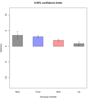
From the table given in the results of using R (toggle above) we see that there are substantial differences
among the three groups for whom Religious Affiliation is known.
We also see that the mean for the Missing subjects is much closer
to the mean of Fundamentalist than to the other means, which
might suggest that Fundamentalists were more likely to refuse to
provide a religious affiliation than were members of the other
groups.
The results of an analysis of variance on Optimism scores of
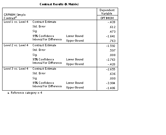
all four groups is presented in Table 2. Here I have asked SPSS
to use what are called "Simple Contrasts" with the last (missing)
group as the reference group. This will cause SPSS to print out a
comparison of each of the first three groups with the Missing
group. I chose to use simple contrasts because I wanted to see
how Missing subjects compared to each of the three non-missing
groups. (In R you need "treatment" contrasts and the first group is the reference group, which is why I used "relevel.")

- Table 2 Analysis of Variance with All Four Groups --
Simple Contrasts
At the top of Table 2 you see the means of the four groups, as
well as the unweighted mean of all groups (labeled Grand Mean).
Next in the table is an Analysis of Variance summary table,
showing that there are significant differences between groups;
(F3,599 = 14.395; p = .000).
A moment's calculation will show you that the difference
between the mean of Fundamentalists and the mean of the Missing
group is 3.094 - 3.533 = -0.439. Similarly the Moderate group
mean differs from the mean of the Missing group by 1.942 - 3.533
= -1.591, and the Liberal and Missing means differ by 0.878 -
3.533 = -2.655. Thus participants who do not give their religious
affiliation have Optimism scores that are much closer to those of
Fundamentalists than those of the other affiliations.
In the section of the table labeled "Parameter Estimates" we
see the coefficients of -.439, 1.592, and -2.655. You should note
that these coefficients are equal to the difference between each
group's mean and the mean of the last (Missing) group. Moreover,
the t values in that section of the table represent a
significance test on the deviations from the mean of the Missing
group, and we can see that Missing deviates significantly from
Moderates and Liberals, but not from Fundamentalists. This
suggests to me that there is a systematic pattern of non-
response which we must keep in mind when we evaluate our data.
Subjects are not missing at random because missingness depends on
the value of that variable. (Notice that the coefficient for
missing is set at 0 and labeled "redundant." It is redundant
because if someone is not in the Fundamentalist, Moderate, or
Liberal group, we know that they are missing. "Missing," in this
case, adds no new information.)
Orthogonal Contrasts
You might be inclined to suggest that the previous analysis
doesn't give us exactly what we want because it does not tell us
about relationships among the three groups having non-missing
membership. In part, that's the point, because we wanted to
include all of the data in a way that told us something about
those people who failed to respond, as well as those who did
supply the necessary information.
I am going to move slightly away from the problem of missing data in order to make this example more complete. If you prefer, you can jump to the next main heading. For those who want to focus on those subjects who
provided Religious Affiliation while not totally ignoring those
who did not, an alternative analysis would involve the use of
orthogonal contrasts not only to compare the non-responders with
all responders, but also to make specific comparisons among the
three known groups. But keep in mind that because the data are
not MCAR the means, particularly the grand mean, is likely to be
biased. (If Fundamentalists are less likely to respond, and if
they have higher optimism scores, the grand mean of optimism will
be biased downward from what it would have been had they
responded.)
You can use SPSS (OneWay) or any other program to perform the
contrasts in question. (Or you can easily do it by hand). Suppose
that I am particularly interested in knowing how the
non-responders differ from the average of all responders, but
that I am also interested in comparing the Moderates with the
other two identified groups, and then the Fundamentalists with
the Liberals. I can run these contrasts by providing SPSS with
the following coefficients.
     Missing vs Non-Missing                          1     1   1     -3
     (Fundamental & Moderate) vs Liberals            1     1  -2      0
     Fundamental vs Liberal                          1    -1   0      0
The first contrast deals with those missing responses that
have caused us a problem, and the second and third contrasts deal
with differences among the identified groups. The results of this
analysis are presented below. (I have run this using SPSS syntax
because it produces more useful printout. The corresponding results from R were given above if you toggled them.)
     ONEWAY
        optimism BY groupnum(1 4)
        /CONTRAST= 1 1 1 -3  /CONTRAST= 1 1 -2  /CONTRAST= 1 -1
        /HARMONIC NONE
        /FORMAT NOLABELS
        /MISSING ANALYSIS .
Table 3 OneWay Analysis of Variance on Optimism with
Orthogonal Contrasts
Notice in Table 3 that the contrasts are computed with and
without pooling of error terms. In our particular case the
variances are sufficiently equal to allow us to pool error, but,
in fact, for these data it would not make any important
difference to the outcome which analysis we used. In Table 3 you
will see that all of the contrasts are significant. This means
that non-responders are significantly different from (and more
optimistic than) responders, that Fundamentalists and Moderates
combined are more Optimistic than Liberals, and that
Fundamentalists are in turn more optimistic than Moderates.
I have presented this last analysis to make the point that you
have not lost a thing by including the missing cases in your
analysis relative to running the analysis excluding missing
observations. The second and third contrasts are exactly the same
as you would have run if you had only used the three identified
groups. However, this analysis includes the variability of
Optimism scores from the Missing group in determining the error
term, giving you somewhat more degrees of freedom. In a sense,
you can have your cake and eat it too, although, as I noted
above, the overall mean is biased relative to what it would have
been had we collected complete data.
Cohen and Cohen (1983, Chapter 7) provide additional comments
on the treatment of missing group membership, and you might look
there for additional ideas. In particular, you might look at
their treatment of the case where there is missing information on
more than one independent variable.
This situation, where data on group membership is missing, is
handled by the analysis above. Notice that, other than the
overall mean, the analysis is not dependent on the nature of the
mechanism behind missingness, which is in fact addressed by the
analysis. This will not necessarily be the case in the following
analysis, where the nature of missingness is important.
1.5 The More General Case of Missing Dependent Variables
We have a different kind of problem when we have data missing
on the dependent variable that makes the results of our study
much more difficult to interpret. If our data are in the form of
a one-way analysis of variance, and if we can assume that data
are missing completely at random, things are not particularly
bad. We will lose power because of smaller sample sizes, and the
means of larger groups will be estimated with less error than
means of smaller groups, but we will not have problems with
biased estimates. But keep in mind that I'm speaking here of data
that are missing completely at random.
But suppose that our data are not missing completely at
random. Suppose that we are comparing two treatments for
hypertension. In the ideal study we have all participants take
the medication they are prescribed and then we compare blood
pressure levels at the end of treatment. But in the real world we
know that there is usually a dropout problem in medical studies.
In particular, those who are not helped by the treatment are more
likely to drop out, or to die. If one drug is quite successful
and the other is pretty much a failure, the final sample size will be
very much smaller in the second treatment. Moreover, those who
remain, and whose blood pressure is eventually measured, are
likely to be the ones who benefitted from the treatment. So if we
see that the means of the two groups are nearly equal at the end
of treatment, we might be led to the conclusion that the two
treatments are equally effective. In fact, one was a horrible
treatment but we didn't have data from its "failures." In such a
setting missing data make the interpretation of means quite
risky. (Perhaps the most appropriate statistic would be the drop
out rate instead of the mean.)
Missing Data Imputation
This is where I am going to split off and create a separate web page on the problem of missing dependent variables. The techniques there are quite a bit more sophisticated that those we have seen so far, but with software that is now generally available, there is much that we can do to salvage our study. To continue, go to Missing data imputation
Alternative Software Solutions
I have shown how to do this with NORM, which is an excellent free-standing program that I recommend. I was asked by a former student if I could write
something that was a step-by-step approach to using NORM, and that document is available
at "MissingDataNorm.html".
You can also do something similar with SPSS and with SAS. In addition, there is an R program called Amelia (in honor of Amelia Earhart). I have written (or will write) instructions for the use of those programs. An important point, however, is that each program uses its own algorithm for imputing data, and it is not always clear exactly what algorithm they are using. For all practical purposes it probably doesn't matter, but I would like to know.
The continuation page for the current page can be found at Missing Data Part Two.
References
Allison, P. D. (2001) Missing Data
Thousand Oaks, CA: Sage Publications.Return
Barladi, A. N. &s;
Enders, C. K. (2010). An introduction to modern missing data analyses.
Journal of School Psychology, 48, 5-37.Return
Cohen, J. & Cohen, P. (1983) Applied
multiple regression/correlation analysis for the behavioral
sciences (2nd ed.).Hillsdale, NJ: Erlbaum. Return
Cohen, J. & Cohen, P., West, S. G. &
Aiken, L. S. (2003). Applied Multiple
Regression/Correlation Analysis for the Behavioral Sciences,
3rd edition. Mahwah, N.J.: Lawrence Erlbaum.
Return
Dunning, T., & Freedman, D.A. (2008)
Modeling section iffects. in Outhwaite, W. & Turner, S.
(eds) Handbook of Social Science Methodology. London:
Sage. Return
Howell,D. C. (2007)
The analysis of missing data. In Outhwaite, W. & Turner, S. Handbook of Social Science Methodology. London: Sage.Return
Little, R.J.A. & Rubin, D.B. (1987)
Statistical analysis with missing data. New York,
Wiley. Return
Jones, M.P. (1996). Indicator and
stratification methods for missing explanatory variables in
multiple linear regression Journal of the American
Statistical Association, 91,222-230. Return
Schafer, J. L. (1997). Analysis of incomplete multivariate data, London, Chapman & Hall.">
Schafer, J.L. & Olsden, M. K.. (1998). Multiple imputation for multivariate missing-data problems: A data analyst's perspective. Multivariate Behavioral Research, 33, 545-571.Return
Scheuren, F. (2005). Multiple imputation:
How it began and continues. The American Statistician,
59, : 315-319.Return
Sethi, S. & Seligman, M.E.P. (1993).
Optimism and fundamentalism. Psychological Science, 4,
256-259. Return

dch: