

This page is a continuation of a document on missing data that I now refer to as Missing Data--Part 1. I have split it off because the document was getting way too long. For those who have not read Part 1, I will repeat the first couple of paragraphs to give the necessary background. If you have read Part 1, you can probably skip to the next main heading. If you would like other examples, I have written a page on logistic regression with missing data. That approach is quite similar to what you do with standard multiple regression, but you might find it useful. The link is Missing-Logistic/MissingLogistic.html
Missing data are a part of almost all research, and we all have to decide how to deal with it from time to time. There are a number of alternative ways of dealing with missing data, and these documents are an attempt to outline those approaches. For a very thorough book-length treatment of the issue of missing data, I recommend Little and Rubin (1987) . A shorter treatment can be found in Allison (2002) . Perhaps the nicest treatment of modern approaches can be found in Baraldi & Enders (2010).
There are several reasons why data may be missing. They may be missing because equipment malfunctioned, the weather was terrible, people got sick, or the data were not entered correctly. Here the data are missing completely at random (MCAR). When we say that data are missing completely at random, we mean that the probability that an observation (Xi) is missing is unrelated to the value of Xi or to the value of any other variables. Thus data on family income would not be considered MCAR if people with low incomes were less likely to report their family income than people with higher incomes. Similarly, if Whites were more likely to omit reporting income than African Americans, we again would not have data that were MCAR because missingness would be correlated with ethnicity. However if a participant's data were missing because he was stopped for a traffic violation and missed the data collection session, his data would presumably be missing completely at random. Another way to think of MCAR is to note that in that case any piece of data is just as likely to be missing as any other piece of data.
Notice that it is the value of the observation, and not its "missingness," that is important. If people who refused to report personal income were also likely to refuse to report family income, the data could still be considered MCAR, so long as neither of these had any relation to the income value itself. This is an important consideration, because when a data set consists of responses to several survey instruments, someone who did not complete the Beck Depression Inventory would be missing all BDI subscores, but that would not affect whether the data can be classed as MCAR.
This nice feature of data that are MCAR is that the analysis remains unbiased. We may lose power for our design, but the estimated parameters are not biased by the absence of data.
Often data are not missing completely at random, but they may be classifiable as missing at random (MAR). (MAR is not really a good name for this condition because most people would take it to be synonymous with MCAR, which it is not. However, the label has stuck.) Let's back up one step. For data to be missing completely at random, the probability that Xi is missing is unrelated to the value of Xi or other variables in the analysis. But the data can be considered as missing at random if the data meet the requirement that missingness does not depend on the value of Xi after controlling for another variable. For example, people who are depressed might be less inclined to report their income, and thus reported income will be related to depression. Depressed people might also have a lower income in general, and thus when we have a high rate of missing data among depressed individuals, the existing mean income might be lower than it would be without missing data. However, if, within depressed patients the probability of reported income was unrelated to income level, then the data would be considered MAR, though not MCAR. Another way of saying this is to say that to the extent that missingness is correlated with other variables that are included in the analysis, the data are MAR.
The phraseology is a bit awkward here because we tend to think of randomness as not producing bias, and thus might well think that Missing at Random is not a problem. Unfortunately it is a problem, although in this case we have ways of dealing with the issue so as to produce meaningful and relatively unbiased estimates. But just because a variable is MAR does not mean that you can just forget about the problem. Nor does it mean that you have to throw up your hands and declare that there is nothing to be done.
The situation in which the data are at least MAR is sometimes referred to as ignorable missingness. This name comes about because for those data we can still produce unbiased parameter estimates without needing to provide a model to explain missingness. Cases of MNAR, to be considered next, could be labeled cases of nonignorable missingness.
If data are not MCAR or MAR then they are classed as Missing Not at Random (MNAR). For example, if we are studying mental health and people who have been diagnosed as depressed are less likely than others to report their mental status, the data are not missing at random. Clearly the mean mental status score for the available data will not be an unbiased estimate of the mean that we would have obtained with complete data. The same thing happens when people with low income are less likely to report their income on a data collection form.
When we have data that are MNAR we have a problem. The only
way to obtain an unbiased estimate of parameters is to model
missingness. In other words we would need to write a model that
accounts for the missing data. That model could then be
incorporated into a more complex model for estimating missing
values. This is not a task anyone would take on lightly. See
Dunning and Freedman (2008) for an
example. However even if the data are MNAR, all is not lost. Our estimators may be biased, but the bias may be small.
I am going to go fairly lightly on what follows, because the solutions are highly technical. I will, however, give references to good discussions of the issues and to software, and I have supplied several examples of the computer code needed to run the analysis on different software program. As implied by the title of this section, the solutions fall into two (overlapping) categories--those which rely on maximum likelihood solutions, and those which involve multiple imputation.
The principle of maximum likelihood is fairly simple, but the actual solution is computationally complex. I will take an example of estimating only a population mean, because that illustrates the principle without complicating the solution.
Suppose that we had the sample data 1, 4, 7, 9 and wanted to estimate the population mean. You already know that our best estimate of the population mean is the sample mean, but forget that bit of knowledge for the moment.
Suppose that we were willing to assume that the population was normally distributed, mainly because this makes the argument easier. Let the population mean be represented by the symbol μ, although in most discussions of maximum likelihood we use a more generic symbol, θ, because it could stand for any parameter we wish to estimate.
We could choose any specific value of μ and calculate the probability of obtaining a 1, 4, 7, and 9 for. This would be the product p(1)*p(4)*p(7)*p(9). You would probably guess that this probability would be very very small if the true value of μ = 10, but would be considerably higher if the true value of μ were 4 or 5. (In fact, it would be at its maximum for μ = 5.25.) You could repeat this for different values of μ, calculate p(1), p(4), etc. and then the product. For some value of μ this product will be larger than for any other value of μ. We want that value of μ that produces the largest probability. We call this the maximum likelihood estimate of μ. It turns out that the maximum likelihood estimator of the population mean is the sample mean, because we are more likely to obtain a 1, 4, 7, and 9 if μ = the sample mean than if it equals any other value. (The maximum likelihood estimate for many other statistics is not necessarily the standard estimate given by the usual statistic estimate.) This is certainly convenient when we have only one variable. In that case we can simply using the sample means and variances. But for more complex problems (which is usually the case), things become messy. What we will carry out is what is called an iterative solution as we audition various potential means and covariances.
I need to add in one "correction" to the solution that I hinted at in the last paragraph. To calculate likelihoods we would have to multiply the probabilities of each of the observed values given a specific set of parameters. But if you multiply a bunch of probabilities you soon come up with a very very small number and lose digital accuracy. So, instead, we take the log of those probabilities and add them. So we are looking for the maximum log likelihood. The logs will be negative, so we want the set of parameters whose log likelihood is closest to 0.0.
If we have multiple variables, we have multiple possible population means. We "audition" various possible sets of values of the parameters. For each possible value or set of values we calculate the likelihood and look for that set of parameters that has the maximum log likelihood. This is fairly straightforward when we have complete data, but when we have missing data we work with those cases with complete data on all variables, then those cases with data missing on variable 1, then those cases with data missing on variables 1 and 2, and so on. To get the likelihood for any vector of means, for example, we sum the log likelihoods over the different sets of variables. Then we move on to another potential vector of means and repeat the process. This continues until we find that vector of means that has the highest (least negative) log likelihood. But then we also have to estimate a matrix of variances and covariances, so you can see that it is not something that you want to carry out by hand.
It is important to point out that at no time in this process do we actually impute any data values, even though I often speak as if we do. What is iterative about this process is that we compute log likelihoods for each auditioned set of parameters, choosing the result with the largest log likelihood. We don't even have to impute data values at the end, because the only purpose of having raw data in any situation is to generate a vector of means and a matrix of variances/covariances, and we already have those at the end of our iterative process.
There are a number of ways to obtain maximum likelihood estimators, and one of the most common is called the Expectation-Maximization algorithm, abbreviated as the EM algorithm. The basic idea is simple enough, but the calculation is more work than you would want to do by hand.
Schafer (1999) phrased the problem well when he noted "If we knew the missing values, then estimating the model parameters would be straightforward. Similarly, if we knew the parameters of the data model, then it would be possible to obtained unbiased predictions for the missing values." Here we are going to do both. We begin with what is called the E-step. We first estimate the variances, covariances and means, perhaps from listwise deletion. (It really isn't all that important what we choose as initial estimates.) We then use those estimates to create a regression equation to predict missing data. (Keep in mind that we would generally need several reqression equations because some variables (due to missing data) will have more or fewer available predictor variables than others.) We then move to the M-step to use those equations to fill in the missing data. (As Enders, 2010, points out, we don't really fill in the missing data, but we can calculate what the variances and covariances would be without actually going through that step. But I speak as if we filled in missing values because I think that it is easier to imagine the process that way.) We then go back to the E-step with our new means and covariances, where we again build regression equations to "fill in" data. Then to an M-step, and on and on until the system stabilizes. At this point we have the necessary means and covariances for any subsequent form of data analysis.
The problem with EM is that it leads to biased parameter estimates and underestimates the standard errors. For this reason, statisticians do not recommend EM as a final solution. Why, then, should I have spent time explaining it? Because it is often used as the first step in procedures that are recommended. So don't give up on EM.
An excellent discussion of the EM algorithm and its solution is provided by Schafer (1997, 1999, and Schafer & Olsen (1998). Schafer has also provided a program that will do EM imputation, as well as other ways of imputing missing data.. That program is named NORM and was freely available from http://www.stat.psu.edu/~jls/misoftwa.html. However, Schafer has moved on to the Census Bureau and that site is gone. But you can download a copy for Windows machines at http://www.uvm.edu/~dhowell/StatPages/Missing_Data/NormProgram.zip. A Web page that I wrote for one of our graduate students on using the stand alone NORM program can be found at MissingDataNorm.html. It covers both the stand-alone program and the R version. This was last updated in late 2012.
The Missing Value Analysis module in SPSS version 13 and later also includes a missing data procedure that will do EM. Their treatment of missing data gets more sophisticated with each version, and, as I write this, they are now up to Version 22.)
An alternative to maximum likelihood is called Multiple Imputation. (Contrary to its normal usage in statistics, "multiple" does not refer to multiple dependent variables, but to multiple data sets generating by repeating the estimation process multiple times.) Each of the solutions that we have discussed involves estimating what the missing values would be, and using those "imputed" values in the solution. For the EM algorithm we substituted a predicted value on the basis of the variables that were available for each case. In multiple imputation we will do something similar, but will add error components to counteract the tendency of EM and Maximum Likelihood to underestimate standard errors.
In multiple imputation we generate imputed values on the basis of existing data, just as we did with the EM algorithm. We begin with an estimate of the means and the covariance matrix, often taken from an EM solution. Using those parameter estimates we replace the missing values with values estimated from a series of multiple regression analyses using the available parameter estimates. (I say a "series" of regression equations because we replace missing data using whatever complete data that subject has, move to the next subject, write a regression equation based upon whatever variables are complete for that subject, and so on. But we want to be sure that we do not underestimate the standard error. If we simply used a straight regression equation, the imputed values would be perfectly determined from the variables included in the analysis and would add no new information. To get around this problem we will use something equivalent to stochastic regression, which adds a bit of random error to each imputed variable.
Assume, for simplicity, that X was regressed on only one other variable (Z). Denote the standard error of the regression as s X.Z. (In other words, sX.Z is the square root of MSresidual.) In standard regression imputation the imputed value of X (X̂) would be obtained as X̂i = b0 + b1Zi. But for data augmentation we will add random error to our prediction by setting X̂i = b0 + b1Zi +ui where ui is a random draw from a standard normal distribution with mean 0 and standard deviation sX.Z. This introduces a degree of uncertainty into the imputed value. Following the imputation procedure just described, the imputed value will contain a random error component. Each time we impute data we will obtain a slightly different result.
Adding a bit of error is our first random component. But there is another random step to be considered. The process above treats the means and covariances, and the associated regression coefficients and standard errors as if they were parameters, when in fact they are sample estimates. But parameter estimates have their own distribution, just as the mean does. (If you were to collect multiple data sets from the same population, the different analyses would produce different values of the estimated parameters, for example, and these estimates have a distribution.) So our second step will be to make a random draw of these estimates from their Bayesian posterior distributions -- the distribution of the estimates given the data, or pseudodata, at hand.
Having derived imputed values for the missing observations, MI now iterates the solution, imputing values, deriving revised parameter estimates, imputing new values, and so on until the process stabilizes. At that point we have our parameter estimates and can write out the first imputed data set.
But we don't stop yet. Having generated an imputed data file, the procedure continues and generates several more data files. (We might iterate the solution 1000 times, writing out an imputed data set after every 200th imputation. By the time we have done another 200 iterations, the data set on which we compute our second data set will be effectively independent of the data for the first data set.) We do not need to generate many data sets, because Rubin has shown that in many cases three to five data sets are sufficient. Because of the randomness inherent in the algorithm, these data sets will differ somewhat from one another. In turn, when some standard data analysis procedure (here we are using multiple regression) is applied to each set of data, the results will differ slightly from one analysis to another. At this point we will derive our final set of estimates (in our case our final regression equation) by averaging over these estimates following a set of rules provided by Rubin.
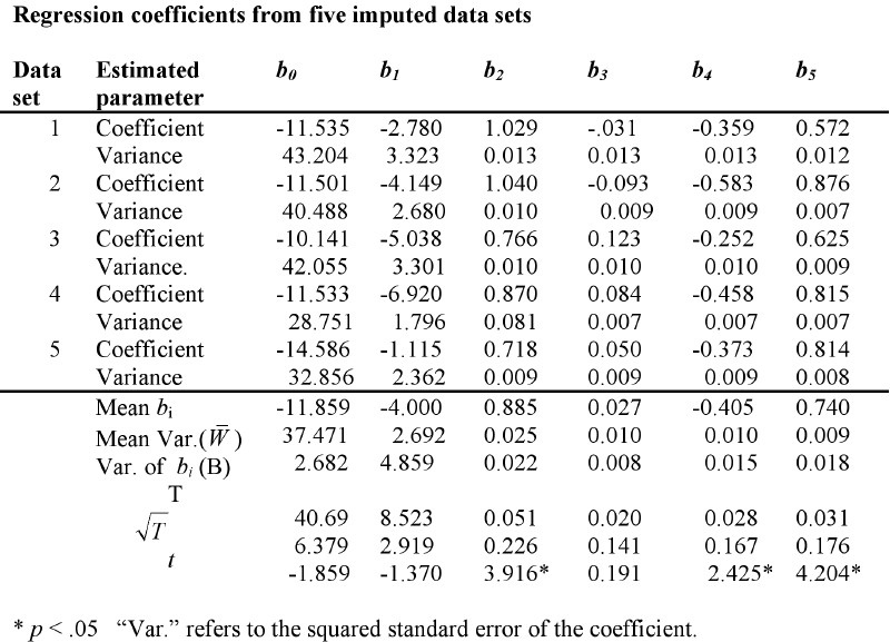
I will illustrate the application of Rubin's method with an example involving behavior problems in children with cancer. The dependent variable is the Total Behavior Problem score from Achenbach's CBCL. The predictor variables are depression and anxiety scores for each of the child's parents, one of whom has cancer. I have used NORM to generate five imputed data sets, and have used SPSS to run the multiple regression of Total Behavior Problems on the five independent variables used previously. These regression coefficients and their squared standard errors for the five separate analyses are shown in the following table.
The final estimated regression coefficients are simply the means of the individual coefficients. Therefore

It is interesting to compare this solution with the solution from the analysis using casewise deletion. In that case

But we also need to pay attention to the error distribution of these coefficients. The variance of our estimates is composed of two parts. One part is the average of the variances in each column. These are shown labeled "Mean Var." in the last row. The other part is based on the variances of the estimated bi. This is shown in the bottom row labeled "Var. of bi." We then define W̄ as the mean of the variances, and B as the variance of the coefficients. Then the Total variance of each estimated coefficient is
T = W̄ + (1 + 1/m)B
where m is the number of imputed data sets.
The values of T and the square root of T, which is the standard error of the coefficient, are shown in the last row of the table. Below them is the result of t = bi √T , which is a t test on the coefficient. Here you can see that the coefficients for the patient's depression score, the spouses depression score, and the spouses anxiety score (predictors 2, 4, and 5) are statistically significant at α = .05. For a somewhat more complete discussion of this process, see the page I have written entitled "MissingDataNorm.html.
The above analysis was carried out with NORM, but I could have used any of several other programs.. I was asked by a former student if I could write something that was a step-by-step approach to using NORM, and that document is available at "MissingDataNorm.html".
You can also do something similar with SPSS and with SAS. In addition, there is an R program called Amelia (in honor of Amelia Earhart). I have written instructions for the use of those programs. The solution using Amelia can be found at Amelia.html. An important point, however, is that each program uses its own algorithm for imputing data, and it is not always clear exactly what algorithm they are using. For all practical purposes it probably doesn't matter, but I would like to know.
- For a page on SPSS, go to MissingDataSPSS.html.
- For SAS, see MissingDataSAS.html.
Apparently I never wrote this section. In its place I recommend a page by Yang Yuan at https://www.ats.ucla.edu/stat/sas/library/multipleimputation.pdf , especially pages 6 - 8.
There is yet a third general solution for missing data which has much to recommend it. It is called Predictive Mean Matching (PMM), and is discussed in an excellent paper by Allison (2015), which is available at https://stats.idre.ucla.edu/r/faq/how-do-i-perform-multiple-imputation-using-predictive-mean-matching-in-r/
(accessed July 9, 2018.). Another good source is https://www.analyticsvidhya.com/blog/2016/03/tutorial-powerful-packages-imputing-missing-values/
Toggle triangle to see a mice.R analysis
> ### Missing Data Using R
> ### /Missing_Data/Missing-Logistic/survrateMissingNA.dat
> # Analysis of missing data using VIM and mice closely following
# the discussion in Kabacoff, 2nd ed., Chapter 158, pp. = 414ff.

setwd("~/Dropbox/Webs/StatPages/Missing_Data/Missing-Logistic")
survival <- read.table("survrateMissingNA.dat", header = TRUE)
head(survival)
survival$outcome01 <- as.factor(survival$outcome01)
library(VIM)    # For visualizaation, not imputation
library(mice)


survival[complete.cases(survival),]
survival[!complete.cases(survival),]
sum(is.na(survival$survrate))
mean(is.na(survival$survrate))
mean(!complete.cases(survival))
md.pattern(survival)

aggr(survival, prop = FALSE, numbers = TRUE)
aggr(survival, prop = TRUE, numbers = TRUE)
matrixplot(survival, axes = TRUE, xlab = "outcome01", ylab = "intrus", interactive = TRUE, labels = TRUE)
marginplot(survival[c("outcome01","intrus")], pch = c(20), col = c("darkgray","red","blue"))
marginplot(survival[c("avoid", "intrus")], pch=c(20),
           col = c("darkgray", "red", "blue"))
x <- as.data.frame(abs(is.na(survival)))
y <- x[which(apply(x,2,sum)>0)]     #Finds x with SOME, not ALL missing
cor(survival, y, use = "pairwise.complete.obs")  #Ignore error message (outcome01 = factor)
imp <- mice(survival,5)
fit <- with(imp, glm(outcome01 ~ survrate + gsi + avoid + intrus, family = binomial))
pooled <- pool(fit)
summary(pooled)
Allison, P. D. (2001) Missing Data
Thousand Oaks, CA: Sage Publications.Return
Barladi, A. N. &s;
Enders, C. K. (2010). An introduction to modern missing data analyses.
Journal of School Psychology, 48, 5-37.Return
Cohen, J. & Cohen, P. (1983) Applied
multiple regression/correlation analysis for the behavioral
sciences (2nd ed.).Hillsdale, NJ: Erlbaum. Return
Cohen, J. & Cohen, P., West, S. G. &
Aiken, L. S. (2003). Applied Multiple
Regression/Correlation Analysis for the Behavioral Sciences,
3rd edition. Mahwah, N.J.: Lawrence Erlbaum.
Return
Dunning, T., & Freedman, D.A. (2008)
Modeling section effects. in Outhwaite, W. & Turner, S.
(eds) Handbook of Social Science Methodology. London:
Sage. Return
Enders, C. K. (2010). Applied missing data analysis. New York; The Guilford Press.
Return
Howell,D. C. (2007)
The analysis of missing data. In Outhwaite, W. & Turner, S. Handbook of Social Science Methodology.
London: Sage.Return
Little, R.J.A. & Rubin, D.B. (1987)
Statistical analysis with missing data. New York,
Wiley. Return
Jones, M.P. (1996). Indicator and
stratification methods for missing explanatory variables in
multiple linear regression Journal of the American
Statistical Association, 91,222-230. Return
Schafer, J. L. (1997). Analysis of incomplete multivariate data,
London, Chapman & Hall.
Schafer, J.L. & Olsden, M. K.. (1998). Multiple imputation for
multivariate missing-data problems: A data analyst's perspective. Multivariate
Behavioral Research, 33, 545-571.Return
Scheuren, F. (2005). Multiple imputation:
How it began and continues. The American Statistician,
59, : 315-319.Return
Sethi, S. & Seligman, M.E.P. (1993).
Optimism and fundamentalism. Psychological Science, 4,
256-259. Return
Last revised 6/26/2015