

Using Vectors in the R Programming Environment
Vector Arithmetic and Examples

The title of this section sounds almost scary, but it really isn't. R uses what is known as "vector arithmetic," which means that it operates on a whole column of data at once. You have seen this elsewhere when I used something like "sqrt(data4)." To explain what I mean, let me go back to the good old days of programming. If you were writing a program in Fortran IV, you would write something like (It's been a long time (nearly 50 years), so the code may be slightly off.)
      do 25 i = 1 to 20
      y(i) = sqrt(x(i))
   25
If you were writing in Pascal, one of my favorites, you would write
   for i := 1 to 20
      do begin
      y(i) <- sqrt(x(i)
    end; {for}
And for C++ it would be
   for (int i = 1; i <= 20; i++) {
	  y(i) = sqrt(x(i)
   }
All of those sets of commands are telling the computer to take each value of x, one at a time, and take its square root. But R doesn't work that way. In one command it tells itself to take the square root of all of the x values. That may not look all that much different, but it is. It is very much faster, especially when you have a lot of values. In the book I do things like take the mean of 10,000 observations. And I can do it in a tiny fraction of a second. Doing it the old way on a much older machine took me 19.5 seconds.
y = sqrt(x)
If you have never done any programming, this may not seem like a big thing. But for those who have, it takes a bit of getting used to. Your commands may look a bit funny to you. Suppose that I really want to take each value of x, multiply it by the corresponding value of y, and store the result. For example, if x = 1, 3, 5 and y = 2, 4, 6, then xy will be equal to 2, 12, 30. But I don't have to go through the list pair by pair. I can just say
   x <- c(1, 3, 5)
   y <- c(2, 4, 6)
   xy <- x*y
   print(xy)
   [1]  2  12  30
Examples From Exercises
I think that I can give you a good idea of just what is going on, and what an R program does, by doing some of the homework exercises in Chapter 2 in one of my books. You don't have to memorize all of these commands, but read them through carefully and understand what they are doing. We can deal with specifics later. Remember, I am not trying to teach you to program in R here. I am just trying to give you some idea of what it will do and roughly what the code looks like. I'll come back to the teaching R bit later.
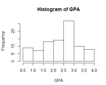
I'll begin with reading in the data in Exercise 2.10. These are in a data file named Ex2-10.dat on the Web site. (You don't need wither of my books to follow this discussion.) Then we will make a stem-and-leaf display of them. Then I will go on to Ex2.12 and Ex2.13, and draw a histogram (at bottom) and stem-and-leaf display. Finally I will go on and do most of Ex2.14 - Ex2-19. The results, shown on the R console, are given below.
d1 <- read.table("http://www.uvm.edu/~dhowell/methods8/DataFiles/Ex2-10.dat",
 header = TRUE)
head(d1)
Sex <- d1$Sex
Grade <- d1$Grade
stem(Grade)

-----------------------------------------------------------
  Sex Grade
1   1    66
2   1    67
3   1    67
4   1    73
5   1    73
6   1    74
-----------------------------------------------------------

stem(Grade) # Or you could use stem(d1$Grade).
-----------------------------------------------------------
  The decimal point is at the |

  66 | 00000
  68 | 0
  70 | 000
  72 | 000000
  74 | 0000000
  76 |
  78 | 0000000000
  80 | 00000000000000
  82 | 0000000000
  84 | 0000000000000
  86 | 0000000000000
  88 | 0000000000
  90 | 00000
  92 | 00000
  94 | 00000
-----------------------------------------------------------
stem(Grade[Sex == 1] )      #Create a subset of grades
-----------------------------------------------------------
  The decimal point is 1 digit(s) to the right of the |

  6 | 677
  7 | 334
  7 | 5999
  8 | 012244
  8 | 5566778
  9 | 23444
  9 | 5
-----------------------------------------------------------
stem(Grade[Sex == 2] )

  The decimal point is 1 digit(s) to the right of the |

  6 | 778
  7 | 00022334
  7 | 55558899999
  8 | 0111111111112222223344
  8 | 5555555666777777888889999
  9 | 00001333
  9 | 5
-----------------------------------------------------------

setwd("~/Dropbox/methods9/DataFiles")
d2 <- read.table("Add.dat", header = TRUE)   # Read in another data frame
head(d2)
-----------------------------------------------------------
  CaseNum ADDSC Gender Repeat  IQ EngL EngG  GPA SocProb Dropout
1       1    45      1      0 111    2    3 2.60       0       0
2       2    50      1      0 102    2    3 2.75       0       0
3       3    49      1      0 108    2    4 4.00       0       0
4       4    55      1      0 109    2    2 2.25       0       0
5       5    39      1      0 118    2    3 3.00       0       0
6       6    68      1      1  79    2    2 1.67       0       1
-----------------------------------------------------------

hist(d2$GPA, breaks = 25)  #breaks controls the number of bars
-----------------------------------------------------------

-----------------------------------------------------------

# Now another stem and leaf display
stem(d2$ADDSC)
-----------------------------------------------------------
  The decimal point is 1 digit(s) to the right of the |

  2 | 69
  3 | 034456679
  4 | 000233444445566677888899999
  5 | 0000000001122333455677889
  6 | 0001223455556899
  7 | 0024568
  8 | 55
-----------------------------------------------------------
### Now some other stuff with vectors

x <- c(10, 8, 9, 5, 10, 11, 7, 8, 7, 7)
y <- c(9, 9, 5, 3, 8, 4, 6, 6, 5, 2)
print(sumx <- sum(x))    # This stores sumx as well as prints it.
[1] 82
print(sumy <- sum(y))
[1] 57
print(sumx2 <- sum(x*x))  # or x2 <- x*x;  sum(x2))
[1] 702
print(sumx.sq <-sum(x)*sum(x))  # or sum(x^2))
[1] 6724
print(n <- length(x))
[1] 10
print(meanx <- sum(x)/n)
[1] 8.2
print(sumy2 <- sum(y*y))  # or y2 <- y*y then  sum(y2))
[1] 377
print(sumy.sq <- sum(y) * sum(y))  # or sum(y^2))
[1] 3249
print(b <- (sumy2 - sumy.sq/n)/(n-1))
[1] 5.788889
print(sumxy <- sumx*sumy)
[1] 4674
print(sumxsumy <- sumx*sumy)
[1] 4674
print(covar <- (sumxy - (sumx)*(sumy)/n)/(n-1))  # This is the covariance
[1] 467.4
print(stdev <- sqrt((sumx2 - sumx^2/n)/(n-1)))
[1] 1.813529
print(sd(x))
[1] 1.813529
>
-----------------------------------------------------------
# Now another stem and leaf display
stem(d2$ADDSC)
-----------------------------------------------------------
The decimal point is 1 digit(s) to the right of the |
2 | 69
3 | 034456679
4 | 000233444445566677888899999
5 | 0000000001122333455677889
6 | 0001223455556899
7 | 0024568
8 | 55
-----------------------------------------------------------
### Now some other stuff with vectors
x <- c(10, 8, 9, 5, 10, 11, 7, 8, 7, 7)
y <- c(9, 9, 5, 3, 8, 4, 6, 6, 5, 2)
print(sumx <- sum(x)) # This stores sumx as well as prints it.
[1] 82
print(sumy <- sum(y))
[1] 57
print(sumx2 <- sum(x*x)) # or x2 <- x*x; sum(x2))
[1] 702
print(sumx.sq <-sum(x)*sum(x)) # or sum(x^2))
[1] 6724
print(n <- length(x))
[1] 10
print(meanx <- sum(x)/n)
[1] 8.2
print(sumy2 <- sum(y*y)) # or y2 <- y*y then sum(y2))
[1] 377
print(sumy.sq <- sum(y) * sum(y)) # or sum(y^2))
[1] 3249
print(b <- (sumy2 - sumy.sq/n)/(n-1))
[1] 5.788889
print(sumxy <- sumx*sumy)
[1] 4674
print(sumxsumy <- sumx*sumy)
[1] 4674
print(covar <- (sumxy - (sumx)*(sumy)/n)/(n-1)) # This is the covariance
[1] 467.4
print(stdev <- sqrt((sumx2 - sumx^2/n)/(n-1)))
[1] 1.813529
print(sd(x))
[1] 1.813529
>
You may have noticed that when I printed out the complete histogram for Grade near the top of the output, the characters on the left were all zeros. But when I printed out the scores for Males, the numbers were quite different. That is simply because of the way that the stem-and-leaf deals with decimal points. The first case treated the value as 66.0, while the second treated it as 66, with the second 6 to the right of the line. Put another way, the first treated the value with a two digit stem to the left, while the second put only one digit for the stem and a second digit for the leaf. Weird!
dch:
Free JavaScripts provided
by The JavaScript Source