
In the 9th edition of Fundamental Statistics for the Behavioral Sciences (2016) I have presented material on using R with direct coding. In this case you enter each of the commands that you want executed, either on the command line or from an editor such as RStudio. I prefer that approach because I think that it is a better way to get across many of the statistical concepts that I cover. But there is another way. If you have any familiarity with SPSS or other mainline statistical packages, you are familiar with its GUI (Graphical User Interface). You know that you select commands from the menu (such as the command to read data) and then SPSS asks you specific questions that set up the procedure to read the data. Or you ask for SPSS to compute a mean, and it gives you a lists of variables from which to chose the one that you want. And people certainly do learn statistics from using SPSS, even if it does operate through a GUI. So why not do the same with R? That is a good question, to which I fall back on the reason I gave above -- I think that it makes the underlying statistical concepts clearer. But some people really do want to use a GUI, and fortunately John Fox, at McMaster University, has written a package called Rcommander (or Rcmdr) that will do just that. The page here is designed to give you a barebones introduction to Rcmdr so that you can pursue it on your own if you wish.
One of the nice things about Rcmdr is how easy it is to start it up. First you want to start R. You can do this either by starting R itself or by starting RStudio, which will, in turn, start R. I think that it is better if you just start the R application itself. That keeps your screen cleaner and easier to navigate. Once you start R you can then simply issue the command "library(Rcmdr)", assuming that you have installed Rcmdr. If you haven't, you first have to type "install.packages("Rcmdr")", and that really isn't too difficult a task.
Note to Mac users. Because of the many graphical features of Rcmdr, it requires what is known as the XQuartz (or X11) windowing system to be installed. Newer version of Mac OS-X do not automatically include X11. When you install Rcmdr it loads extra things, and my MacPro, which did not have X11 installed, worked fine after installing Rcmdr. However, if you have problems, you can go to http://xquartz.macosforge.org to install it. That's probably a good thing to do anyway.
Now that you have started R and Rcmdr, you will have two windows that look like :
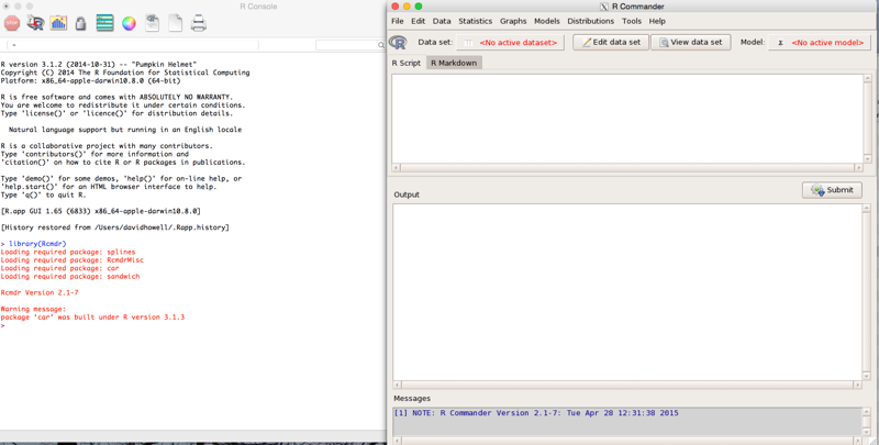
In the very lower right of the RCommander window you see a funny bit of stuff. You drag that to change the size of the screen. We are going to carry out most of our work from the tool bar at the top . But first let's consider the two screens. The one of the left is the standard R screen, and you can pretty much ignore this if you are issuing all of your commands through Rcmdr. Feel free to go ahead and cover it up. The window on the right is the R Commander window, on which we will do most of our work. I will explode that window so that we can better see its elements.
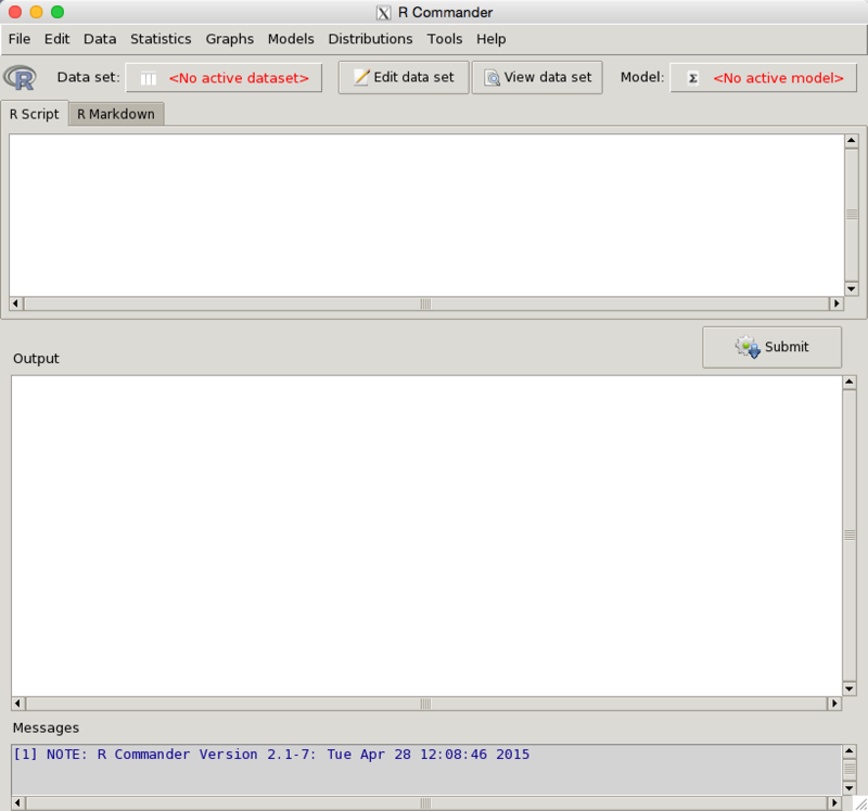
At the top you see a menu bar which includes elements like "Data", "Statistics", Graphs", and so on. That is where you will do much of your work. Below that is a tool bar that allows you to make changes to your data. Near the bottom is a "submit" button, which you will click once you have instructed the program what you want done. (It is like the "Run" button in RStudio.)
First we need to load some data. But be careful, because you want to "import" data, not "load" it. Loading is something else--its loads R datasets that have been created by R on a previous run. So go to data/import/from text file, etc. on the menu bar, give the name of the data frame that this will be creating (e.g.MRdata), and click "open." That will issue the code that will import those data. Notice that there is a small box indicating that the variable names are at the top of the file. For any of my data files, make sure that this is checked. Then, let's make sure that you loaded the right data by click on View Data Set in the tool bar. That will show you a small spreadsheet view of your data. That's all there is to it. Notice that nothing has appeared on the R window. That's fine. The command to load the data was entered in the top window of Rcmdr and echoed when we clicked the submit button in the lower window.
Suppose that you have a small file that you want to enter by hand. There are two ways of doing this. One is to enter the R command yourself. Simply go to the Rcmdr window and type varA <- c(23, 36, 43, 23, 45, 7). Then click on the submit button. Then type varA in the Rcmdr window, click submit, and the data will be printed out in the lower window. Or you can use Rcmdr's data entry system by clicking on Data/New data set in the menu bar, give the data set a name, tell it to create the necessary rows and columns, and enter your data. I find this more work than I like, so I would use the first command that I gave.
I can't go through everything that Rcmdr will do, but I can give you a few examples and you can take it from there. (I give some excellent online references below.) One of the first examples that I use in the text is found in a file named Tab3-1.dat. We can load that as I did above, calling it MRdata because it contains data on mental rotation.
Before continuing, you need to take into account that some of the variables are factors and some are numeric. When R sees the Stimulus and Response variables, it knows that they are factors because they are text. But Accuracy is coded 0 and 1, so it could be numeric. But we know that 0 and 1 stand for "wrong and "right," so we want to make it plain that Accuracy is a factor. So you want to go to Data/Manage variables in active data set/Convert numeric variables to factors. You will then be asked to specify what 0 and 1 stand for. That is the only variable there that I would recode as a factor (the two others were classed as factors automatically), so we are done with that.
Now let's learn something about the variables; for example, their means. So go to Statistics/Summaries/Numeric Summaries. I selected RTsec. I wanted to break those means down by Accuracy, so I went ahead and selected that under Summarize by:. I clicked OK and obtained the following:
Variable: RTsec
          mean        sd  IQR   0%  25%  50%  75% 100%   n
Wrong 1.755636 0.6609498 0.56 0.72 1.38 1.53 1.94 3.45  55
Right 1.611266 0.6344541 0.72 0.72 1.12 1.53 1.84 4.44 545
Notice that mean reaction time is greater for incorrect responses.
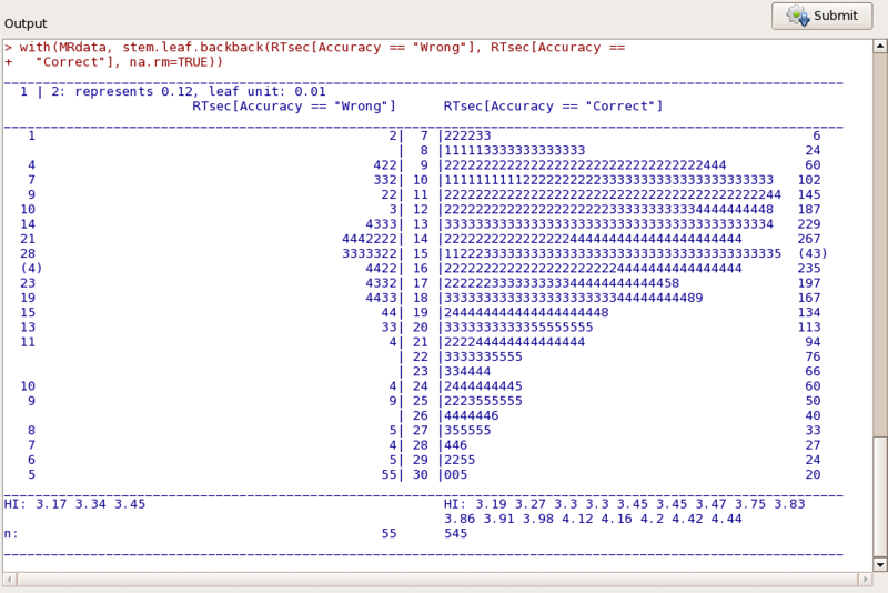
Now lets graph the data. I'll simply make a stem-and-leaf of RTsec. Just select Graphs, Stem-and-Leaf, choose RTsec as the dependent variable and request a back-to-back plot using Accuracy. (But note: make sure that you have first made Accuracy a factor, and you may need to click the reset button before specifying the variables to plot.). Now ask it to create the plot. You will obtain the following in a separate window.
Once we have the data read into Rcmdr we would likely want to know something about each of them. The simplest way to do that is to use Statistics/Summaries/Numerical Summaries. There are other summaries that we could use, but showing you one should be enough . Suppose that we want the mean and standard deviation of RTsec. Choosing that will give us:
> numSummary(MRdata[,"RTsec"], statistics=c("mean", "sd", "IQR",
 "quantiles"), quantiles=c(0,.25,.5,.75,1))
   mean        sd    IQR   0%  25%  50%    75% 100%   n
 1.6245 0.6377245 0.7625 0.72 1.12 1.53 1.8825 4.44 600
That's not very exciting, but it does give us those statistics along with the quartiles. Suppose instead that we wanted to create a contingency table of Accuracy and Stimulus. This would address the question about whether the person is more accurate in his response dependng on whether the stimulus has only been rotated, or if it is a rotated mirror image. I'm sure that you can figure out how to ask for that from the statistics menu. The result follows.
Frequency table:
         Stimulus
Accuracy  Mirror Same--
  Wrong       12     43
  Correct    286    259

	Pearson's Chi-squared test

data:  .Table
X-squared = 18.7845, df = 1, p-value = 1.464e-05
It looks as if the subject is more often wrong when the stimululs is a mirror image of the original. That doesn't particularly surprise me.
I think that you can figure out most of the rest under the statistics menu. Just try out a bunch of things. But there is one thing that may confuse people, especially if they come across it early in the book. Suppose that we want to run a multiple regression or an analysis of variance. To over-simplify, they are basically the same analysis except that for regression the predictors are continuous variables, while in the analysis of variance they are categorical. But to do either of them, we have to go through two steps. First we have to create a model (of the form y ~ x1 + x2 + x1*x2). Once that is created we ask R to convert that to a regression table or an analysis of variance table. So first create the model.
If you want to do a multiple regression, go to Statistics/fit models/linear regression. Then you simply indicate the role of each variable. (The response variable is RTsec, and explanatory variables are Angle and Trial.) The results follow.
> summary(RegModel.1)

Call:
lm(formula = RTsec ~ Angle + Trial, data = MRdata)

Residuals:
     Min       1Q   Median       3Q      Max
-1.04370 -0.39032 -0.09605  0.27069  2.38892

Coefficients:
              Estimate Std. Error t value Pr(>|t|)
(Intercept)  1.8761561  0.0591239  31.733  < 2e-16 ***
Angle        0.0023566  0.0003994   5.901 6.06e-09 ***
Trial       -0.0015433  0.0001325 -11.651  < 2e-16 ***
---
Signif. codes:  0 '***' 0.001 '**' 0.01 '*' 0.05 '.' 0.1 ' ' 1

Residual standard error: 0.5616 on 597 degrees of freedom
Multiple R-squared:  0.227,	Adjusted R-squared:  0.2244
F-statistic: 87.64 on 2 and 597 DF,  p-value: < 2.2e-16
That is not a very exciting analysis because I only had two continuous variables that made sense. But you can see what happens. Note that this model is called RegModel.1. If we now wanted confidence intervals on the regression coefficients, we would make sure that the RegModel.1 is selected on the right of the toolbar, and then we would go to models/confidence intervals/ and run that. The result is shown below.
> Confint(RegModel.1, level=0.95)
                Estimate        2.5 %       97.5 %
(Intercept)  1.876156086  1.760039872  1.992272300
Angle        0.002356588  0.001572274  0.003140902
Trial       -0.001543258 -0.001803386 -0.001283130
If we had used categorical variables to create LinearModel.2, using the same approach as above but with categorical variables, , we would take LinearModel2 and go to Statistics/Hypothesis tests/ Anvoa table. You can try that out to see what results. Then try some of your other choices.
I am going to leave my coverage of Rcmdr at this point. My goal was to show you how to start it and how to use the menu structure. You can experiment to your heart's content, and I hope that you do. One way to do that would be to take the examples in the book and see if you can repeat them. Do not expect that it will work every time. But after you have figured out what you did wrong, you will have learned something important.
There is a lot of material on the web that will help you master RCommander. John Fox and Milan Bouchet-Valat have written a good manual that is available at http://socserv.mcmaster.ca/jfox/Misc/Rcmdr/Getting-Started-with-the-Rcmdr.pdf. Another good source, also much more complete than what I have written, can be found at http://users.monash.edu.au/~murray/stats/BIO3011/Rmanual_paper.pdf. Natasha Karp has a very good page at http://cran.r-project.org/doc/contrib/Karp-Rcommander-intro.pdf I recommend all of these.
dch