Markov models

Markov models
Markov models are mathematical models of sequential processes. They are used in many ways and in many disciplines, from market or weather prediction to reconstruction of phylogenetic trees. They are often used to model phenomena that change over time with certain statistical regularities.
In their structure, they are quite simple. One form of Markov model, a Markov chain, can be represented as a single square matrix.
\begin{bmatrix} 0.30 & 0.22 & 0.48\\ 0.14 & 0.71 & 0.15\\ 0.05 & 0.64 & 0.31\\ \end{bmatrix}
What’s this all about? A Markov model consists of a finite set of states, and a finite set of transitions between states. To continue with the example above, notice that the matrix is square, 3 \times 3. Each entry in the matrix represents the probability of moving from one state to another. How many states are there? Three. If we have three states, then to account for all possible transitions between states, we need three transitions from each state, and this gives us our matrix. To make this more clear, we can label the rows and columns of the matrix:
\begin{array}{c|ccc} & A & B & C \\ \hline A & 0.30 & 0.22 & 0.48 \\ B & 0.14 & 0.71 & 0.15 \\ C & 0.05 & 0.64 & 0.31 \\ \end{array}
Each entry corresponds to a transition between states, with some probability. With this model, for example, if we’re in state A, there’s a 0.22 probability of transitioning to state B.
We can represent this model as a state diagram. A state diagram is a graph, in which each node represents a state, and each directed edge represents a transition between states. Here’s a rendering of the model above as a state diagram.
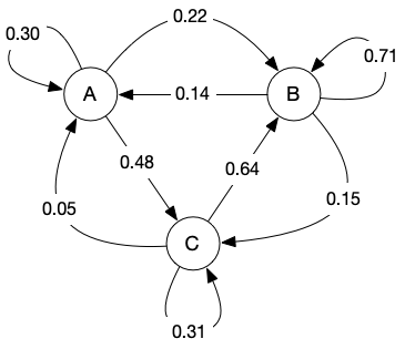
The matrix representation and the state diagram are strictly equivalent. There’s no information in one that is not in the other.
So what do the states A, B, C represent? We haven’t said, but Markov models can be used in many contexts. Let’s say these three states represent our friend Egbert’s choices for listening to music, letting A represent “jazz”, B represent “indie”, and C represent “avant-garde.” So under this model, if Egbert is currently listening to jazz (state A), there’s an 0.30 probability the next album chosen will be another jazz album (again in state A), an 0.22 probability that he’ll switch to indie (state B), and an 0.48 probability he’ll listen to avant-garde next (state C). Given whatever Egbert is listening to right now, we can use this model to predict what genre he’ll listen to next.
So what makes this model a Markov model? A Markov model is
- purely stochastic—transitions between states are based on probability alone,
- “memoryless”—the future state of the model depends only on the current state and the transitions associated with that state, without any memory of the sequence of transitions that led to the current state.
We often refer to these constraints as the Markov property. Given the present state, any past or future states are independent. Markov models are memoryless, stochastic processes. Hence, we often refer to the matrix for a Markov model as a stochastic matrix (we also, equivalently, call this a transition matrix). These models are useful when we have phenomena that can be decomposed into states, with well-defined transition probabilities.
Notice also that each row in a stochastic matrix must sum to one. This must be the case, because each row represents probabilities of transitioning from a specific state to all states (including, possibly, itself). If all rows don’t sum to one, something is wrong.
Even with these constraints, Markov models can exhibit some interesting behaviors and make useful predictions.
There are many types of Markov model, but they all share these common properties.
Varieties of Markov model include:
- Markov chains (discrete time, observable),
- hidden Markov models (HMMs; models with “hidden” states),
- Markov decision processes (which incorporate actions and rewards),
- continuous-time Markov chains (CTMCs),
- and others.
Copyright © 2023–2026 Clayton Cafiero
No generative AI was used in producing drafts of this material. This was written the old-fashioned way. AI was used to rewrite existing pseudocode in LaTeX to produce standalone *.tex files for rendering, and for revisions toward satisfying WCAG 2.1 AA-level accessibility standards as required by UVM policy. AI may also have been used to proofread selected human-written prose. Claude 2.1 with model Sonnet 4.6. Revisions, if any, were performed by the author. AI was not used in generating any code whatsoever. All code samples and starter code are by the author only.