Markov decision process

Author

Clayton Cafiero

Published

2026-06-22

A Markov decision process (MDP) is a mathematical framework for modeling decision-making in situations where outcomes are partly random and partly under the control of a decision-maker. In other words, they formalize sequential decision-making under uncertainty. MDPs are widely used in fields like reinforcement learning, Q-learning, operations research, recommendation systems, autonomous agents, and robotics.

MDPs model an agent interacting with an environment over time. Agents could be robots, drones, players of games, or many other types of agent. At each time step, the agent has some information about the state of the environment, and based on this the agent takes some action—moving left or right, up or down, buying or selling shares in a market, etc. Each action has associated with it a reward or penalty. Rewards or penalties will vary depending on context. The goal of an MDP is to maximize rewards over time—not just near-term rewards, but cumulative rewards over time.

Key components

A set of states (S): Represents all the possible configurations or situations the system can be in.
A set of actions (A): The well-defined set of actions or decisions available to the agent at each state.
Transition probability (P): The probability of moving from one state to another, given a particular action. This captures the uncertainty in outcomes.
- P(s' \mid s, a) is the probability of transitioning to state s' from state s after taking action a.
Rewards (R): The immediate reward received for being in a state or performing an action in a state.
Policy (\pi): A strategy that tells the agent which action to take from each state to maximize rewards over time.
Discount factor (\gamma): A value between 0.0 and 1.0 that determines how much future rewards are valued compared to immediate rewards.

The goal

The objective in an MDP is to find a policy that maximizes the cumulative reward (often called the expected return or utility) over time. If future rewards are discounted (which is typical), the return is computed as:

\mathcal{U} = R_0 + \gamma R_1 + \gamma^2 R_2 + \gamma^3 R_3 + \ldots

where R_t is the reward at time t and \gamma is the discount factor.

Why “Markov”?

MDPs have the Markov property: the probability of transitioning to a new state, and the reward received, depend only on the current state and action—not on the sequence of states and actions that preceded it. As a result, an agent’s policy need only consider its current state, not its entire history, in order to act optimally. (We will, however, need to consider future states to completely evaluate a given state, but that’s a different matter, as we will see shortly.) Recall also that MDPs allow us to model decision-making under uncertainty, so they naturally incorporate stochasticity as well as determinism.

A simple model

Let’s take, for example, a simple environment with an agent.

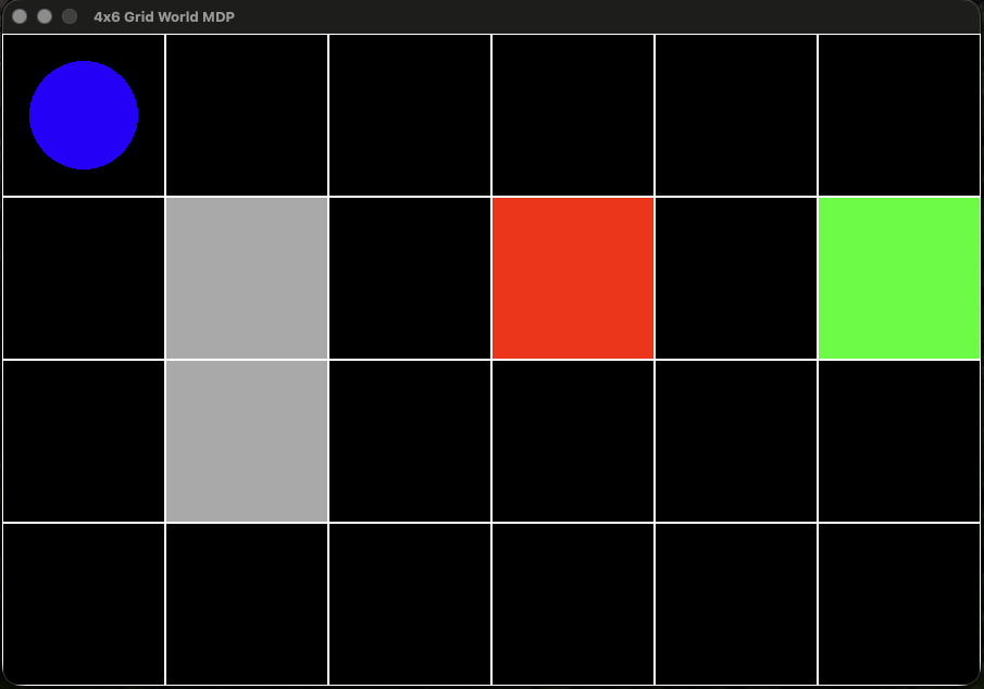
Here the agent—a robot—is represented by a blue circle. The environment is divided into grid cells. There is a barrier shown in grey, a hazard shown in red, and another cell marked in green. If the robot reaches the green cell, it receives a big reward. If the robot navigates into the hazard, it’s game over. The robot may travel orthogonally within the grid, but it may not pass through any barrier (moves into the barrier are blocked). The green square has a high reward; the red has a large negative reward (penalty).

Randomness enters the scene in this way: if the robot chooses to move in a given direction, it actually moves in that direction with a probability less than one. It may also slip side-to-side, moving orthogonally to the intended direction. Anyone who’s ever operated a radio-controlled toy car knows that real landscapes are uneven, and cars don’t always go in the direction you tell them to.

An MDP allows us to solve for a policy that directs the agent in such a way that reward is maximized over time. Let’s say our robot will get a big reward for reaching the green square—say it’s a charging station. A shortest path is easy to solve for, but it might not represent the best route for maximizing reward. Why? Because there’s a risk of falling into the hazard. Recall there’s some randomness here—the robot may not always travel in the intended direction. Accordingly, the safest policy—the one that maximizes expected reward—may well be to travel around the barrier and approach the charging station from the south (assuming north is at top in our diagram). Whether or not this is the case depends on the system of rewards and penalties.

An optimal policy

A policy tells the agent what action to perform when in a given state. In our gridworld example, the states are the robot’s position on the grid. So a policy would tell the robot: if you’re on such-and-such a square on the grid, perform action X, where X in this case is one from among the set of possible moves: go north, go south, go east, or go west.

Here’s the system of rewards we’ll use:

Default reward: -0.1 (any move has a small negative reward, you may think of this as consuming battery power)
Hazard: -100.0 (big negative reward)
Charging station: +10.0

Let’s also assume that if we try to move in a given direction in the absence of barriers we have a 0.8 probability of moving in the intended direction and a 0.1 probability for each of the orthogonal directions (left or right of intended direction).

Under this scenario, we arrive at this policy:

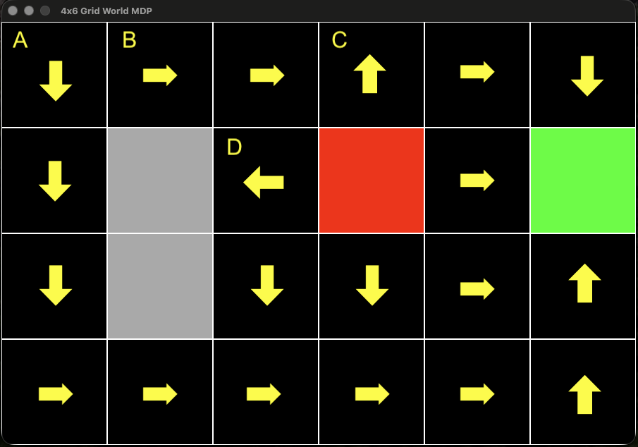
Most of these moves make sense. If we’re at square A, it makes sense to move south to skirt the barrier, but if we’re already at square B, it makes sense to continue to the east. But what’s going on at squares C and D? In these cases, the model has seen the steep penalty of falling into the hazard (maybe it’s liquid hot magma).

The model has also seen that if it decides to move east, there’s a non-zero probability of moving south. Thus, if at square C, it makes sense—if the magma is hot enough—to tell its navigation system to move north. Of course, it can’t move north, since the gridworld is bounded, but it has a 0.1 chance of moving east and a 0.1 chance of moving west, but a 0.0 chance of moving south and falling into the hazard. Similarly, if at square D, it’s safer not to try to move north or south to get away from the hazard but rather to tell the navigation system to go west, thus guaranteeing that it won’t fall into the hazard.

Notice there’s no reference to a starting point, just a recommended action based on where the agent finds itself within the environment. Notice also that if we were at square A, then the recommended policy would not take us along the shortest path, but on a longer, safer route.

Pretty clever, right?

Now let’s see how we can solve for an optimal policy.

Solving for an optimal policy—the Bellman equation

To solve for an optimal policy, we need several things:

a transition model,
a reward model,
a discount factor, and
an environment.

The transition model tells us the probability of getting from some state s to state s', given action a, and we write P(s' \mid s, a). In other words, this is the probability of reaching state s' conditioned upon being in state s and performing action a. We must have an element in our transition model for each state / action pair.

The reward model is a function which gives us the reward—positive, negative, or zero—received by reaching state s' from state s by taking action a. We may write this R(s, a, s'), or merely R(s) if there’s no difference in a reward based on the action that got us to a given state. Again, there should be an element in the reward model for each state in the system.

We also need a discount factor. The discount factor, usually written \gamma, tells the model how to discount future rewards. It’s a concept common in finance. A dollar today is worth more than a dollar a year from now (except under bizarre conditions). Why? Because of inflation, and because we might be able to invest the dollar now and have something more to show for it in a year’s time. The discount factor is necessarily in the interval [0.0, 1.0], though typically it’s in the range between 0.50 and 0.95 (varies with problem instance). With \gamma = 1.0, there’s no discounting at all (very unusual), and with \gamma = 0.0, we’re completely disregarding any future rewards (also unusual).

We refer to the discounted sum of rewards for a sequence of states as the utility of the sequence, and we write

\mathcal{U}(s_0, s_1, s_2 \ldots, s_k) = R(s_0) + \gamma R(s_1) + \gamma^2 R(s_2) + \ldots + \gamma^{k} R(s_k),

and thus, for an infinite sequence we have

\mathcal{U}(s_0, s_1, s_2 \ldots) = \sum\limits_{t=0}^\infty \gamma^t R(s_t).

We denote a policy with a lower-case \pi (no, here it’s not 3.1415\ldots) and we denote an optimal policy as \pi^{*}. So the utility of some policy \pi for some state s is given by

\mathcal{U}^{\pi}(s) = E \bigg(\sum\limits_{t=0}^\infty \gamma^t R(s_t)\bigg).

That is, under policy \pi, the utility of state s is the expected reward of that state plus the expected sum of the discounted rewards of all subsequent states reachable from s. Here E(\cdot) denotes expected value. Because transitions are stochastic, following \pi from s doesn’t trace out a single fixed sequence of states. Rather, it induces a distribution over possible sequences. Thus, \mathcal{U}^\pi(s) is the average of \sum_{t=0}^\infty \gamma^t R(s_t) over that distribution.

An optimal policy is one which chooses the arguments that maximize utility over all possible policies.

\pi^{*} = \underset{\pi}{\operatorname*{arg\,max}}\, \mathcal{U}^{\pi}(s)

The optimal action at a state is given by

\pi^{*}(s) = \underset{a \in A(s)}{\operatorname*{arg\,max}} \sum\limits_{s'} P(s' \mid s, a)\,\mathcal{U}(s').

where A(s) is the set of all possible actions from state s and s' is reachable from s by action a. Thus, the utility of a given state s is

\mathcal{U}(s) = R(s) + \gamma\,\underset{a \in A(s)}{\operatorname*{max}}\sum\limits_{s'} P(s' \mid s, a)\,\mathcal{U}(s').

This is the Bellman equation, and there’s a lot going on so let’s unpack it.

\mathcal{U}(s) is the cumulative utility at state s.
R(s) is the current reward at state s.
\gamma is the discount factor applied to future rewards.
\underset{a \in A(s)}{\operatorname*{max}} gives the value of the best action at state s. That is, it gives the greatest expected utility achievable from s.
\sum\limits_{s'} P(s' \mid s, a) is where stochasticity enters. It’s the sum over all states.
\mathcal{U}(s') is recursive. It calculates the utility of child states.

Value iteration

One method for solving for an optimal policy is called value iteration. Value iteration is an algorithm to find the optimal value function \,\mathcal{U}^{*}(s) (the utility function defined above) in an MDP by iteratively applying the Bellman optimality equation.

The optimal value function \,\mathcal{U}^{*} is given by

\mathcal{U}^{*}(s) = \underset{\pi}{\max}\,\mathcal{U}^{\pi}(s),

that is, the optimal value function returns the best value we can get from any given state, s.

As noted earlier, to do this we must have a complete model:

a well-defined set of states,
a well-defined set of actions available at each state,
a transition model P(s' \mid s, a) (probability of reaching state s' from s taking action a),
a reward function: R(s, a, s') and R(s) (default), and
the discount factor, \gamma.

Here’s how it works:

Initialize value function \,\mathcal{U}(s) to arbitrary values (usually zeros).
The iteration step:
- for each state s:
  - for each possible action a available at s:
    - compute the expected utility of the states s' reachable from s by taking action a, using the current values: \sum\limits_{s'} P(s' \mid s, a)\,\mathcal{U}(s').
  - take the action a that maximizes this sum—this is the \underset{a \in A(s)}{\operatorname*{max}} term in the Bellman equation—and use it to compute an updated value for s: \,\mathcal{U}'(s) = R(s) + \gamma\,\underset{a \in A(s)}{\operatorname*{max}}\sum\limits_{s'} P(s' \mid s, a)\,\mathcal{U}(s').
  - track how much the value of s changed: \Delta = \max(\Delta,\ \lvert \,\mathcal{U}(s) - \mathcal{U}'(s) \rvert).
- once every state s has been visited, replace \,\mathcal{U}(s) with \,\mathcal{U}'(s) for all s simultaneously. (The old values \,\mathcal{U}(s') are used throughout an entire sweep—updates aren’t applied one state at a time as we go. This is sometimes called a synchronous update.)
Repeat step 2, resetting \Delta = 0 at the start of each sweep, until \Delta < \theta for some small threshold \theta.
Return \,\mathcal{U}(s), which at this point approximates \,\mathcal{U}^{*}(s) for every state s.

Two kinds of cells need special handling throughout this process:

Terminal states—like the charging station and the hazard in our gridworld—have no outgoing actions to consider. Their value is fixed at \mathcal{U}(s) = R(s) from the start, and step 2 simply skips over them.
Obstacles—like the barrier—aren’t states the agent can occupy at all, so they’re skipped too.

Once \,\mathcal{U} has converged to \,\mathcal{U}^{*}, recovering the optimal policy takes one more pass over the states. We can recover an optimal policy directly from \,\mathcal{U}^{*} using the formula given earlier:

\pi^{*}(s) = \underset{a \in A(s)}{\operatorname*{arg\,max}} \sum\limits_{s'} P(s' \mid s, a)\,\mathcal{U}^{*}(s').

That is, having found the long-run value of every state, the best action at s is simply whichever action leads, in expectation, to the highest-value successor states.

Running this algorithm on our gridworld—with \gamma = 0.9 and \theta = 10^{-4}—produces the value function \,\mathcal{U}^{*} and the policy shown earlier. Each arrow in that policy diagram is the result of this final arg-max step.

One detail is worth dwelling on: the transition model P(s' \mid s, a) has to account for what happens when the agent’s intended (or slipped) direction would carry it off the grid or into a barrier. In that case, the agent simply stays where it is, so that probability mass is assigned to s' = s rather than to some neighboring cell. This is exactly what’s going on at squares C and D in our earlier example: the probability of “moving” into a wall isn’t lost, it’s redirected to staying put.

No generative AI was used in producing drafts of this material. This was written the old-fashioned way. AI was used to rewrite existing pseudocode in LaTeX to produce standalone *.tex files for rendering, and for revisions toward satisfying WCAG 2.1 AA-level accessibility standards as required by UVM policy. AI may also have been used to proofread selected human-written prose. Claude 2.1 with model Sonnet 4.6. Revisions, if any, were performed by the author. AI was not used in generating any code whatsoever. All code samples and starter code are by the author only.

Reuse

CC BY-NC-SA 4.0