Adversarial games

There was a time when the “holy grail” of AI research was developing a chess-playing program that could beat a grandmaster. In 1996, IBM’s Deep Blue became the first computer program to defeat a world champion under tournament regulations. Gary Kasparov won the match, but Deep Blue won two games (4–2). In a rematch in the following year, Deep Blue won the match 3½–2½ (a tie is scored as ½ for each player). Kasparov was not happy about this; the folks at IBM were thrilled.
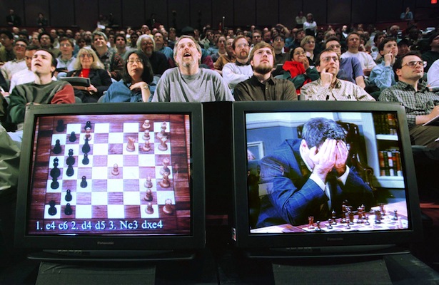
Why chess? People have long thought that chess—especially at the grandmaster level—represents a test of intellectual prowess. It requires a deep understanding of the history of the game, of strategy, of tactics. It requires an ability to look ahead beyond the current move and to anticipate the actions of an opponent. It requires an ability to correctly choose good moves among a great many possible moves. In a word, it requires intelligence, at least by some measure.
As a result, a tremendous amount of AI research has been invested in approaches to playing adversarial games. Having an opponent “raises the bar”, so to speak, on the difficulty of finding solutions. It’s not enough to solve a puzzle, one has to contend with an opponent who’s trying to defeat them with every move.
It’s not just chess that is of interest. Almost every adversarial game has rules, strategies, and tactics worth exploring.
The subject of adversarial games is large, so we will narrow our focus. But before we do, let’s see different ways we can classify adversarial games.
Adversaries
By definition adversarial games are those which involve an adversary or adversaries—opponents. Some games are strictly two player games: classical chess, checkers, backgammon, tic-tac-toe, mancala, Battleship, go, and many others. Some games are multi-player games in which there may be three or more players: Monopoly, Catan, Yahtzee, Chinese checkers, many card games, etc.
We will focus on two player games.
Turn-taking
Many adversarial games are turn-taking games, but many others are not. Turn-taking games include checkers and Battleship. Games that aren’t turn-taking include many role-playing games (especially computer-based role-playing games) and games in which two or more players work to achieve some objective in a limited amount of time, for example, given a multiset of letters, find the most dictionary words that can be constructed from letters in the multiset, or an Easter egg hunt.
We will focus on turn-taking games.
Observability
Observability refers to how much information players have about the game state. A game may be fully-observable or partially-observable. Games in which a player or players have incomplete information about the game state are partially-observable. For example, there are many guessing games—I Spy, Twenty Questions, Mastermind, or Who Am I?— where one (or perhaps more) players start with very little information and then gain information over time. Most card games are partially-observable: gin rummy, poker, blackjack. Some board games are partially-observable: Battleship, for example. Observability may refer to many aspects of a game—the position of an opponent’s pieces or rewards or hazards, certain “powers” or weapons in role-playing games and so on.
Many games are fully-observable, where opponents (and indeed, onlookers) can see the entire game state. Such games include chess, checkers, Connect 4, Othello, Quarto, go, backgammon, and many others. Everyone sees the board (or game state), everyone has the same information.
We will focus on fully-observable games.
Determinism
Some games are entirely deterministic, that is, there is no element of chance and changes in game state are fully determined by players’ moves. Deterministic games include chess, Battleship, and checkers, for example.
Other games are not fully deterministic, and we refer to them as non-deterministic. These are games that incorporate some element of chance. The role chance plays can vary. Sometimes it determines a player’s move—roll the dice and advance so many squares. Sometimes chance limits a player’s move—for example in backgammon, where the available moves are restricted by the state of the pieces on the board and a roll of the dice. Sometimes chance is introduced by shuffling cards or spinning a wheel.
We will take up the subject of non-deterministic games later, but at first we’ll focus on deterministic games.
Zero-sum and non-zero-sum games
A zero-sum game is a game in which one player’s gain is exactly the other player’s loss—gain and loss sum to zero. Other games, including those where both players can gain points may be non-zero-sum games. This is a subject of great interest in game theory, but we will set this aside for the most part.
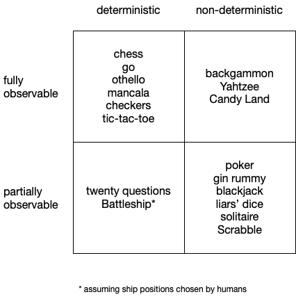
A classification of games
Here’s a classification of some games along two axes: fully-observable vs partially-observable on one axis, deterministic vs non-deterministic on the other.
What’s special about adversarial games?
When we investigated heuristic search, we were concerned with finding a goal node within some graph. Now, a goal node may well represent a winning configuration in a game, but with adversarial games we cannot just search for a goal node and then follow the path to the goal node. Why? Because our adversary is performing actions intended to keep us from reaching such a configuration. Indeed, our adversary wishes to find their own path to a game state that represents a win for them.
So \astar isn’t really suited for this kind of problem. We’ll need a different kind of approach.
When playing against an opponent—or writing a computer program to play against an opponent—we don’t want to count on poor play, mistakes or blunders on the part of our opponent. The only rational strategy for finding our best move is to assume optimal play on the part of our opponent. It is only under this assumption that we’ll find the best moves for ourself.
In order to do this, we’ll need some way of evaluating game states. But how do we do this with two players, each of whom is trying to win? We’ll need a way of assigning some value to board positions that somehow captures the strength of a player’s position. It makes sense to do this in a way such that one player is always trying to maximize this score, while the other player is trying to minimize this score. Consider the most rudimentary (and incomplete) set of evaluations:
| Score | Significance |
|---|---|
| 1 | MAXIMIZING player wins |
| 0 | tie |
| -1 | MINIMIZING player wins |
Now this set of evaluations clearly applies to the end of the game only—either the maximizing player has won, the minimizing player has won, or the game has ended in a tie. We refer to game states in which the game is over as terminal states. When representing the game as a graph, we’ll refer to the nodes corresponding to these terminal states as terminal nodes. This is a start, but it doesn’t help us to determine a player’s best moves before a terminal state is reached. For this, we’ll need some way of evaluating non-terminal nodes. We’ll refer to the evaluation of a given game state (or node associated with a given game state) as a static evaluation—evaluation at a particular point in a game.
If you’ve ever played chess, you’re probably familiar with a common, naive approach to static evaluation: counting point weights assigned to pieces and subtracting one player’s sum from their opponent’s sum. For example, a common system is given by the following table:
| Type of piece | Weight |
|---|---|
| queen | 9 |
| rook | 5 |
| bishop | 3 |
| knight | 3 |
| pawn | 1 |
We exclude the king, because the king can never be removed from the board. Now, of course, this scheme leaves a lot out. For example, a rook isn’t worth much if it’s hemmed in by pawns and a knight as it is at the start of a game. A “pinned” piece may not be able to move at all. A piece may be attacking or poised to attack, in which case it might be worth more than indicated here. A pawn in starting position isn’t worth as much as one that’s poised to move into the opponent’s back rank and thus be promoted. There’s much more that might go into an evaluation (and indeed good chess programs do exactly that), but let’s look at one static evaluation.
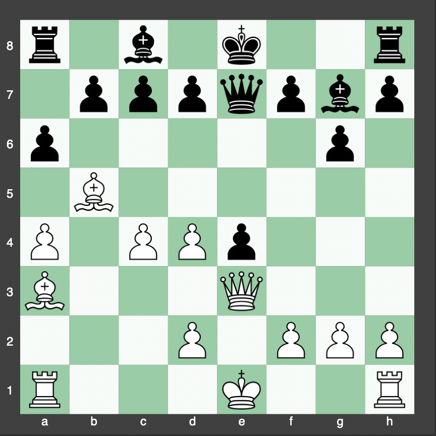
In this state, white has a queen, both rooks, both knights, and seven pawns. Summing the given point weights that gets us 9 + (2 \times 5) + (2 \times 3) + (7 \times 1) = 9 + 10 + 6 + 7 = 32 for white. Black has the following material: one queen, two rooks, two bishops and eight pawns. That’s 9 + (2 \times 5) + (2 \times 3) + (8 \times 1) = 9 + 10 + 6 + 8 = 33. To get the evaluation of this board from white’s perspective, we subtract 33 from 32 and get -1. White is down one pawn and has a material disadvantage. Notice that this evaluation does not consider that white threatens black’s queen or that black threatens white’s bishop (and many other factors). It’s naive, but it illustrates the point: white should be taking steps to maximize this score, black should be making moves that minimize it.
There’s nothing special about positive and negative here except for the fact that each player seeks to push the score as far from the origin as possible in their respective direction. We could reverse signs and roles, and the situation would be exactly the same.
Now we’re ready to learn how to determine a player’s best move (or moves) using an algorithm called “minimax”.
Copyright © 2023–2026 Clayton Cafiero
No generative AI was used in producing drafts of this material. This was written the old-fashioned way. AI was used to rewrite existing pseudocode in LaTeX to produce standalone *.tex files for rendering, and for revisions toward satisfying WCAG 2.1 AA-level accessibility standards as required by UVM policy. AI may also have been used to proofread selected human-written prose. Claude 2.1 with model Sonnet 4.6. Revisions, if any, were performed by the author. AI was not used in generating any code whatsoever. All code samples and starter code are by the author only.