Alpha-beta pruning

Speeding up minimax with \alpha–\beta pruning
We’ve seen that in all but the most trivial of games, generating the entire game tree for evaluation is impractical at best and often quite impossible. What is done instead is we generate only a portion of the tree. However, even generating a portion of the tree can be expensive. We have the same time complexity as we saw with \astar: \mathscr{O}(b^d) where b is the branching factor and d is the depth of our search. This includes the cost of generating and evaluating nodes.
We want our game-playing engine to be both fast and strong. The deeper the search, the better the engine can choose among possible moves. At the same time, the deeper our search, the higher our cost, both in terms of time and space. There’s a real tradeoff here.
But what if we didn’t have to generate and evaluate so many nodes? If we could ignore certain nodes or subtrees, then we could probe to greater depth elsewhere in the same amount of time, or we could achieve the same level of play in shorter time. Sounds good, right?
It turns out there’s a technique for doing exactly this called \alpha–\beta pruning. This algorithm keeps track of the best score of which MAX is guaranteed given the evaluations so far, and the best score of which MIN is guaranteed given the evaluations so far. Under certain conditions, we can use this information to determine whether a node or subtree can possibly change our evaluation at the root node. If it cannot, we don’t expand the node or subtree, and we don’t evaluate. So “pruning” is a bit of a misnomer. It’s not the case that we generate nodes and then prune them—instead we don’t generate them at all.
Let’s build an intuition first.
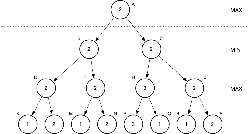
Consider this partial game tree with MAX to move and depth limit three.
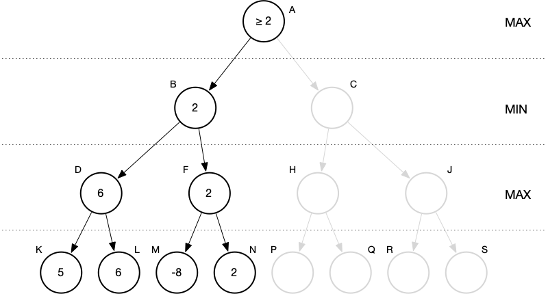
Before we ever get to the right subtree we know one thing to a certainty: whatever MAX’s best score can be, it can’t possibly be less than two. MAX is guaranteed at least a score of two. Why? Let’s say that at node C, the right child of A, the value worked out to be less than two. MAX wouldn’t choose the move represented by node C. MAX would have a better move at node B—the one with a score of two.
If the score at node C worked out to be greater than two, then MAX would make the move represented by node C, because it would have a better score. But that doesn’t change the fact that with only the left subtree evaluated we’d know that MAX was guaranteed at least a score of two.
So far so good?
Now let’s consider this scenario.

While exploring the right subtree, we generate nodes C, H, P, and Q. We evaluate P and Q and find scores of 0 and -1 respectively. H gets the maximum of these: zero. But now what do we know at node C? Remember, node C represents a move for MIN. With node H evaluated, MIN is guaranteed a best score of zero. No matter what’s in the right subtree under C, MIN is guaranteed no worse than zero. Now, MAX’s guaranteed minimum score is 2 and MIN’s guaranteed maximum score is 0. At the root, with incomplete information, MAX would choose the move represented by node B.
Now ask yourself: Are there any values at all for nodes J, R, or S that could possibly change this decision?
No. There are not. There are no values for these nodes that could change the outcome—none whatsoever. Let’s verify.
Say we found values that would lead to a value at J of greater than two.

Does this change MAX’s decision? No, it does not.
Now say we found values that would lead to a value at J of less than zero.
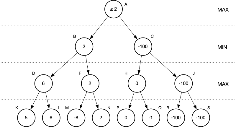
Does this change MAX’s decision? No, it does not. So at this point…
MAX has all the information needed to choose the best move. It does not matter at all what’s in the subtree rooted at J.
Accordingly, when this kind of scenario occurs, we don’t bother generating any additional children of C—we don’t need to because it won’t change the outcome a whit. Any additional subtrees of C are “pruned.”
So how do we know when we can prune and when we cannot? This is where \alpha and \beta come in. \alpha is just a variable we use to keep track of the guaranteed best score so far for MAX, and \beta just keeps track of the guaranteed best score so far for MIN. If ever we reach a point where \alpha \geq \beta we can prune.
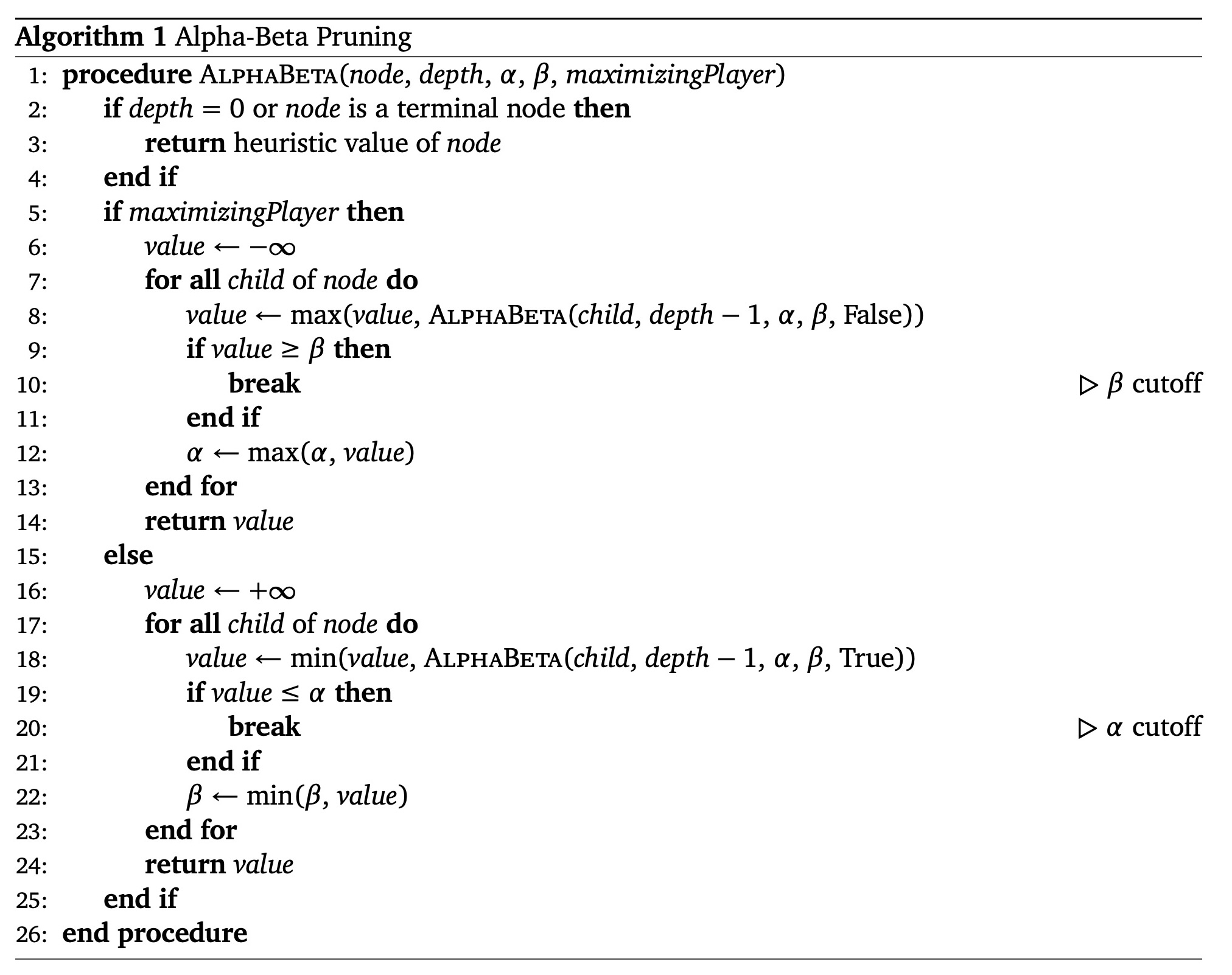
Modifying the minimax algorithm to make use of \alpha–\beta pruning is straightforward. We initialize \alpha to be negative infinity (if the language supports it) or some very large negative number (if the language does not support infinity), and similarly, we initialize \beta to be positive infinity. As the algorithm proceeds, we update \alpha and \beta as needed.
Some practice problems for minimax with \alpha–\beta pruning
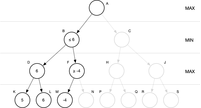
Problem 1: Do we need to descend into the right subtree of A or can we prune?
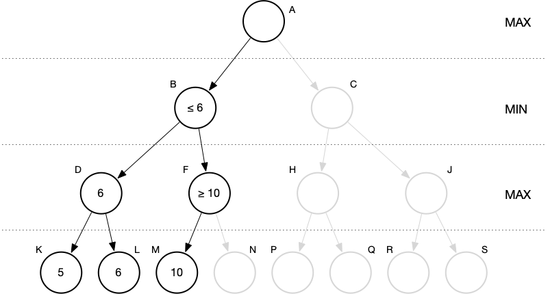
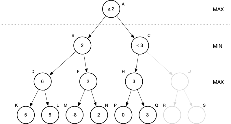
Problem 2: Do we need to look at the right child of F or can we prune?
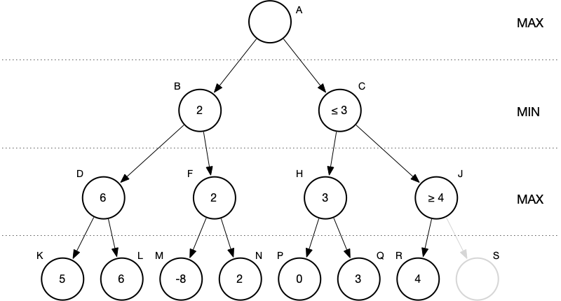
Problem 3: Do we need to descend into the right subtree of C or can we prune?
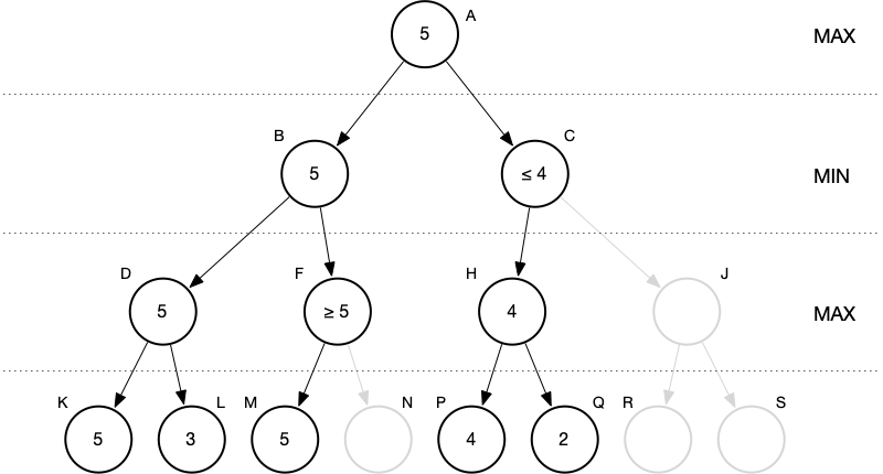
Problem 4: Do we need to look at the right child of J or can we prune?
There’s always a “gotcha”
There’s always a “gotcha” and \alpha–\beta pruning is no exception.
\alpha–\beta pruning is sensitive to the ordering of evaluations. When the best moves are evaluated first, we have tight bounds for \alpha and \beta which can result in significant pruning. In the best case, with “perfect” ordering, we get \mathscr{O}(\sqrt{b^{d}}) = \mathscr{O}(b^{d/2}). In the worst case, where bad moves are evaluated first we’re stuck with \mathscr{O}(b^{d}). So there’s a huge difference between perfect ordering and worst ordering. In real-world applications, we usually get something between these extremes, and there’s only tiny computational overhead for tracking \alpha and \beta and performing comparisons so there’s no reason not to use \alpha–\beta pruning.
In these two small examples we can see minimax’s sensitivity to order. In the first, with “good” order, only five static evaluations are performed. In the second, with “bad” order, it’s eight of eight.
Why don’t we just generate nodes for the best moves first? Because if we knew the best moves in advance there’d be no reason to use minimax at all, with or without pruning! The whole point is that we don’t know in advance.
There are different approaches to improve minimax including iterative deepening, heuristics, and hash tables, but these are for another day.
Copyright © 2023–2026 Clayton Cafiero
No generative AI was used in producing drafts of this material. This was written the old-fashioned way. AI was used to rewrite existing pseudocode in LaTeX to produce standalone *.tex files for rendering, and for revisions toward satisfying WCAG 2.1 AA-level accessibility standards as required by UVM policy. AI may also have been used to proofread selected human-written prose. Claude 2.1 with model Sonnet 4.6. Revisions, if any, were performed by the author. AI was not used in generating any code whatsoever. All code samples and starter code are by the author only.