IDA Star

The No Free Lunch theorem

The No Free Lunch theorem states (informally) that no single algorithm is best for all possible cases. An algorithm that performs well in one context may perform poorly in others. There are always trade-offs.

The same is true for \astar.

The problem with \astar

We’ve seen that the worst case for \astar is the same as the worst case for Dijkstra’s algorithm—\mathscr{O}(\lvert V \rvert^2), where V is the size of the vertex set. However, we’ve seen that in most cases \astar outperforms Dijkstra, requiring fewer dequeue operations. So what’s the problem?

The problem is space. We often focus on the time complexity of an algorithm because this is often the most significant limitation. However, a \mathscr{O}(n \log n), for example, isn’t much use if its space complexity is too high, say \mathscr{O}(n^5). In a case like this, the algorithm is fast, but it consumes tremendous amounts of memory. An algorithm is useless if it runs out of memory in all but the smallest problem instances.

The space complexity of \astar depends on the average branching factor and the depth of search required to find the goal. The branching factor of a graph is simply the number of edges divided by the number of non-leaf vertices. Depth measures the number of edges traversed from some starting node (the root in a tree) to another given node. If we have a branching factor of, say, three, and a depth of five, and if we explore all branches that’s 3^5 = 243 branches. In general, if the branching factor is b and the depth is d, that’s b^d. Obviously this grows exponentially.

Branching factor

Since \astar maintains a priority queue, the worst case space complexity for \astar is \mathscr{O}(b^d). That’s not great. In fact, there are many problems for which this becomes a serious issue.

Take, for instance, a Rubik’s Cube. You might think we could represent this as a graph, and treat it as a graph search problem. In that you’d be correct, but consider the space needed if we were to try to use \astar. The branching factor of a Rubik’s Cube is between 13 and 14, and the depth from any arbitrary starting point to a solution by the smallest number of steps is about 20. The space needed for finding a solution using \astar would be on the order of 10^{22} entries in the priority queue. Yeah. Good luck with that.

So what’s to be done?

\idastar: Iterative deepening \astar

There’s an approach that uses significantly less memory called \idastar or iterative deepening \astar. But in order to understand this, we must first understand how uninformed iterative deepening depth-first search works (IDDFS). One we understand IDDFS, we can add heuristics and modify the algorithm to use the additional information.

Iterative deepening depth-first search

The space problem of \astar isn’t unique. \astar, Dijkstra’s algorithm, and even plain-vanilla breadth-first search all share the same \mathscr{O}(b^d) worst-case space complexity.

At first, IDDFS may sound preposterous, but bear with me.

IDDFS is like depth-first search (DFS), except we probe only to a fixed depth and go no further. Say we’re searching a tree for some goal node and we want to recover the full path of how we reached the goal node. IDDFS would go about it like this:

Let the depth limit equal zero. Is the root node the goal node? No? Then increment depth limit to one and run DFS all over again, starting from the root node. Did we find the goal node at depth one? No? Then increment depth limit to two and run DFS all over again, starting from the root node. We keep doing this until we find the goal node or some other stopping criterion is reached.

Sounds crazy, right? Isn’t this really inefficient? Actually, it’s not as bad as you might think.

Consider the number of paths that exist at a given depth, and the number of times we expand (explore) each level in our search tree.

Depth	Number of paths at that depth	Number of times a node is expanded at that depth	Total number of paths
1	b	d	db
2	b^2	d - 1	(d - 1)b^2
3	b^3	d - 2	(d - 2)b^3
\vdots	\vdots	\vdots	\vdots
d - 1	b^{d-1}	2	2b^{d-1}
d	b^d	1	b^d

The important point here is that the tree is expanded most often at depth one—where there are fewer branches, and the depth at which we have the most branches is expanded only once. Let that soak in: We expand few branches many times, and many branches few times.

The total number of expansions is

b^d + 2b^{d-1} + \dots + (d - 2)b^3 + (d - 1)b^2 + db + (d + 1) = \sum\limits_{i=1}^d (d + 1 - i)b^i.

If we factor out b^d, we get

b^d(1 + 2b^{-1} + 3b^{-2} + \dots + (d - 1)b^{2-d} + db^{1 - d} + (d + 1)b^{-d}).

Let x = b^{-1}, and substitute in and we get

b^d(1 + 2x +3x^2 + \dots + (d - 1)x^{d-2} + dx^{d - 1} + (d + 1)x^d).

Furthermore, we have this inequality

b^d(1 + 2x +3x^2 + \dots + (d - 1)x^{d-2} + dx^{d - 1} + (d + 1)x^d) < b^d(1 + 2x + 3x^2 + \dots)

and

b^d(1 + 2x + 3x^2 + \dots) = b^d \sum\limits_{n=1}^{\infty} nx^{n - 1}.

This converges to

b^d \frac{1}{(1 - x)^2}.

But notice that \frac{1}{(1 - x)^2} does not depend on depth (recall that x = b^{-1}), so this is a constant term. And what do we do with constant terms in asymptotic analysis? We disregard them! So that means that the time complexity of IDDFS is (drum roll, please) \ldots

\mathscr{O}(b^d).

Depth-first search and IDDFS have the same time complexity (up to that constant factor)! Crazy, right? But there you have it.

But what’s the space complexity? Here’ where we get the big payoff. Like DFS, IDDFS uses a stack and not a queue as its supporting data structure. What’s the space complexity? It’s linear in the depth of the search: \mathscr{O}(d)! The stack only keeps track of the current path we’re exploring.

\idastar: Iterative deepening \astar (for real this time)

Now that we’ve seen how IDDFS works, let’s see how we can add a heuristic and adapt it accordingly. Our objective is not to probe the tree (or graph) to a fixed depth at each iteration, but rather to probe more promising paths to a greater depth than we do unpromising paths. We’ll still take an iterative approach, increasing the “depth” of our searches along each branch in a systematic way.

Here’s how it works.

1. Calculate the f-score, f(x) = g(x) + h(x) for the start node. Since g(\text{start}) = 0 by definition, this amounts to the heuristic for the start node. This is the threshold value used to determine when to stop probing.

2. In a loop, until a goal node is found:

   1. Perform DFS as usual, but keep track of the f-scores for nodes visited along a given branch.
   2. Keep probing until the goal is found or a node is encounted which exceeds threshold. Once such a node is encountered, stop probing on that branch.
   3. If the current iteration is exhausted without finding the goal, set the threshold to a new value—the smallest of the f-scores exceeding threshold in the last iteration.

In this way, we probe to variable depth depending on the threshold value.

Example

Consider this graph. Edge costs are indicated on the edges. Heuristics are shown in red just outside of each node. Let’s do \idastar step-by-step.

\idastar example

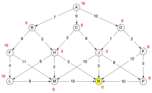
First, let’s verify that the heuristic is admissible and consistent.

Admissibility check

Node	h(x)	h^*(x)	h(x) \leq h^*(x)?
A	16	17	YES
B	9	10	YES
C	8	8	YES
D	9	10	YES
F	16	21	YES
H	5	5	YES
J	3	3	YES
K	8	15	YES
L	16	18	YES
M	9	10	YES
P	8	10	YES
N	0	0	YES

The heuristic is admissible. No node overestimates the true cost to the goal N.

Consistency check

Edge	h(x)	c(x, y) + h(y)	h(x) \leq c(x, y) + h(y)?
A \to B	16	7 + 9 = 16	YES
A \to C	16	9 + 8 = 17	YES
A \to D	16	10 + 9 = 19	YES
B \to F	9	8 + 16 = 24	YES
B \to H	9	5 + 5 = 10	YES
C \to H	8	3 + 5 = 8	YES
C \to J	8	8 + 3 = 11	YES
D \to J	9	7 + 3 = 10	YES
D \to K	9	2 + 8 = 10	YES
F \to L	16	4 + 16 = 20	YES
F \to M	16	11 + 9 = 20	YES
H \to L	5	6 + 16 = 22	YES
H \to M	5	2 + 9 = 11	YES
H \to N	5	5 + 0 = 5	YES
J \to M	3	10 + 9 = 19	YES
J \to N	3	3 + 0 = 3	YES
J \to P	3	8 + 8 = 16	YES
K \to P	8	5 + 8 = 13	YES
K \to N	8	12 + 0 = 12	YES
L \to M	16	8 + 9 = 17	YES
M \to N	9	10 + 0 = 10	YES
P \to N	8	10 + 0 = 10	YES

The heuristic is consistent. All edges satisfy the triangle inequality.

Trace

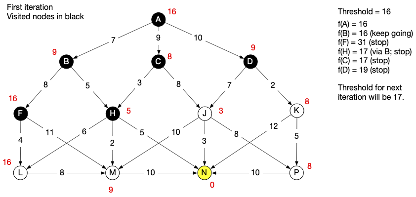
To get started, we see that f(A) = g(A) + h(A) = 0 + 16 = 16, so we set our initial threshold to 16. Then we start depth-first search and keep track of the smallest f-score that exceeds the current threshold. When we encounter a node for which the threshold is exceeded we stop probing on that branch. We will proceed by conventional left-first traversal order, but it would work just as well with right-first.

First iteration

We don’t find the goal on the first iteration, so we update the threshold to equal the smallest f-score above threshold in the previous iteration. We run again with threshold of 17.

Second iteration

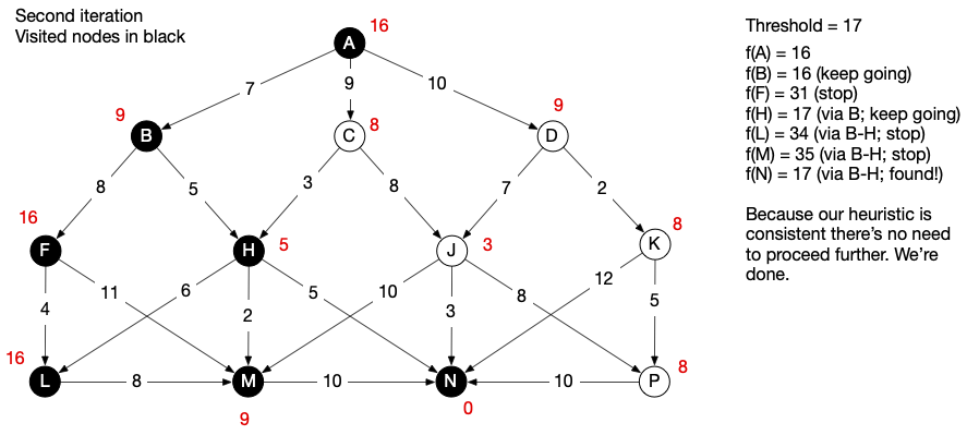
Now we find the goal node, at a cost of 17. Because our heuristic is consistent, once we’ve found the goal, we know the path we’ve found must be a lowest-cost path, so we terminate search and recover the path from breadcrumbs A \to B \to H \to N. It’s straightforward to confirm that this is indeed a lowest-cost path.

Copyright © 2023–2026 Clayton Cafiero

No generative AI was used in producing drafts of this material. This was written the old-fashioned way. AI was used to rewrite existing pseudocode in LaTeX to produce standalone *.tex files for rendering, and for revisions toward satisfying WCAG 2.1 AA-level accessibility standards as required by UVM policy. It may also have been used to proofread selected human-written prose. Claude 2.1.150 with model Sonnet 4.6. Revisions, if any, were performed by the author. AI was not used in generating any code whatsoever. All code samples and starter code are by the author only.