
Link
Patches are areas at least 8% below normal covering 5 acres or more. A patch's tier is the highest class covering at least 5 acres of it. Each cell shows acres, with the number of patches in parentheses.
Click a row to see the patch on the map.
The table follows the year and area chosen here. The graph shows every year for the area.
Product
Year
Visible Layers
No aerial survey data for this year yet.
This is a screening layer: it shows where the canopy was browner than usual, not why. About these data
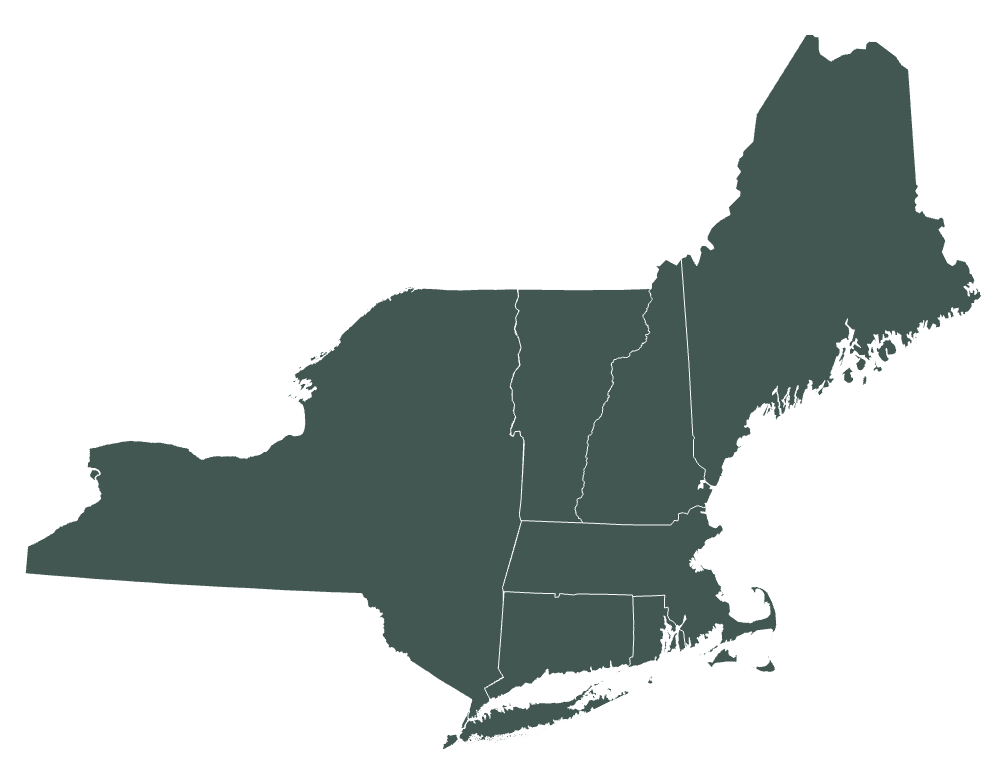
Welcome! The Remote Sensing maps of the Northeastern Forest Health Atlas (NEFHA) use satellite imagery to show where the forest canopy across the Northeastern US was less green than usual, and how forest greenness has changed from year to year. They complement the Atlas's aerial survey maps: aerial surveys record damage that trained observers saw from the air and attributed to a cause, while these maps measure canopy greenness across all forest, every growing season, at 10-meter resolution.
Two products are available. The greenness deficit (NE-FGDN) shows how far each patch of forest fell below its own normal in a given season, with larger affected areas outlined as disturbance patches. SenTrendr shows each location's greenness for every year since 2017, so you can see when canopy was lost and whether it is coming back.
Users can choose a product, year and state, shade the map by deficit class or another classification method, overlay same-year aerial survey outlines, compare with dated satellite imagery, click any location or patch to see its greenness history, and list the most severe patches by state.
These maps are preliminary screening tools. They show where the canopy changed, not why, so please read the FAQ tab before drawing conclusions. This project is administered by the Forest Ecosystem Monitoring Cooperative.
For information on acceptable use of this data, see the Data Policy tab.
Aerial detection surveys have long been the backbone of forest health monitoring in the Northeast, but they capture only what is visible from aircraft, on the days and over the areas flown each year. Since 2017, the European Union's Copernicus Sentinel-2 satellites have imaged the whole region every few days at 10-meter resolution1, making it possible to follow canopy condition across all forest, every growing season.
The Remote Sensing maps measure canopy greenness with NDVI, the normalized difference vegetation index2. Healthy leaves absorb red light and strongly reflect near-infrared light; when leaves are eaten, browned, thinned or removed, NDVI drops. Comparing greenness against what is normal for each location is an established way to flag forest disturbance, used at coarser resolution by the US Forest Service's ForWarn system3. Following each location's greenness through a stack of yearly images is the idea behind LandTrendr4, which SenTrendr adapts to Sentinel-2's finer 10 m pixels.
The maps are built in Google Earth Engine from Sentinel-2 surface reflectance, with clouds and shadows removed using Google's Cloud Score+5. Forest is identified with Google's Dynamic World land cover6 and the USGS National Land Cover Database7.
See the Methods tab for how each product is calculated, and the FAQ tab for important caveats to understand when using these maps.
References
1 Drusch, M., et al. 2012. Sentinel-2: ESA's optical high-resolution mission for GMES operational services. Remote Sensing of Environment 120: 25-36.
2 Tucker, C.J. 1979. Red and photographic infrared linear combinations for monitoring vegetation. Remote Sensing of Environment 8: 127-150.
3 Hargrove, W.W., Spruce, J.P., Gasser, G.E. and F.M. Hoffman. 2009. Toward a national early warning system for forest disturbances using remotely sensed canopy phenology. Photogrammetric Engineering & Remote Sensing 75: 1150-1156.
4 Kennedy, R.E., Yang, Z. and W.B. Cohen. 2010. Detecting trends in forest disturbance and recovery using yearly Landsat time series: 1. LandTrendr, temporal segmentation algorithms. Remote Sensing of Environment 114: 2897-2910.
5 Pasquarella, V.J., Brown, C.F., Czerwinski, W. and W.J. Rucklidge. 2023. Comprehensive quality assessment of optical satellite imagery using weakly supervised video learning. Proceedings of the IEEE/CVF Conference on Computer Vision and Pattern Recognition Workshops: 2125-2135.
6 Brown, C.F., et al. 2022. Dynamic World, near real-time global 10 m land use land cover mapping. Scientific Data 9: 251.
7 Dewitz, J. 2023. National Land Cover Database (NLCD) 2021 Products. U.S. Geological Survey data release.
A full technical methods document is in preparation.
Frequent looks. Sentinel-2 flies two satellites, so each spot is imaged at least every 5 days, and every 2 to 3 days across much of the region where neighboring passes overlap. A May-September season brings roughly 30 to 70 looks at each 10 m pixel.
Clouds are removed pixel by pixel. Cloud Score+ rates how clear every 10 m pixel is in every image. Pixels scoring below 0.60, and those the image's own classification marks as cloud or shadow, are dropped. A mostly cloudy scene still contributes its clear gaps, so what matters is how often each spot was clear, not how many cloudless days there were. Over 2017-2022 a typical pixel had about 96 clear observations, roughly 16 per season.
Medians, not averages. Some haze and shadow slips past any cloud screen, and it always makes forest look browner. Both products use medians, which one bad image cannot drag down: 0.84, 0.85, 0.86, 0.83 and a hazy 0.52 have a median of 0.84 but an average of 0.78.
Timing. The greenness deficit compares each clear observation with the pixel's expected greenness on that exact date, so it does not matter which days were clear. SenTrendr's single yearly median does depend on timing: if a cloudy summer leaves mostly May leaf-out observations, that year reads slightly low. Treat small year-to-year changes in SenTrendr (about 0.02 NDVI) as noise; large drops are real.
Where coverage is thin. 2017 (one satellite for the first part of the year), unusually cloudy seasons, and the edges of satellite passes have fewer clear observations and are noisier. The greenness deficit needs at least two clear observations in a three-week window and usually at least three usable windows in a season; pixels with less are left blank.
Imagery. Every clear Sentinel-2 surface reflectance observation from May through September, with clouds and shadows removed using Cloud Score+, converted to NDVI at 10 m.
The normal. For each pixel, a smooth seasonal curve is fitted to every clear May-September observation from 2017 to 2022. The curve is fixed and never refitted, so every year is compared against the same reference. Pixels with fewer than 20 clear observations in those years are left blank.
The season's deficit. Each clear observation in a later season is expressed as a percent of the curve on its own date. The season (May 1 to September 1) is split into six windows of about three weeks, and each window keeps the median of its observations (at least two are needed), which resists a single hazy image. The deficit is the average, over the windows, of how far that median sat below 100% of normal. 0 means at or above normal; greening is not mapped.
Forest only. A pixel counts as forest if Dynamic World mapped it as trees in at least 5 of the years 2018-2024, excluding developed land and open water in the 2021 National Land Cover Database. A stand cleared in 2023 therefore stays in the mask, so its loss shows in later years.
Deficit classes. Low (2-8% below normal), moderate (8-21%), high (21-45%) and very high (45% or more), set from natural breaks in the deficit across the region. The names describe how far greenness fell, not how much damage occurred. Less than 2% is treated as normal and not drawn.
Disturbance patches. Pixels at least 8% below normal are joined into patches of 5 acres or more. A patch's tier is the highest class covering at least 5 acres of it. Where a patch overlaps same-year aerial survey damage by 20% or more of its area, the most-overlapping damage agent is reported.
Years and states. 2024, 2025 and 2026, for all seven states.
Yearly greenness. For each 10 m pixel and each year from 2017 to 2026, the median NDVI of all clear May-September Sentinel-2 observations, with the same cloud screening as the greenness deficit.
Forest only, but looser. A pixel is included if Dynamic World mapped it as trees in the first or the last year of the record, excluding open water. Developed land is deliberately not removed, so forest that became buildings or pavement stays in and its conversion shows.
Patch histories. For each greenness-deficit disturbance patch, the yearly greenness of all its pixels is summarized as an average, percentiles and a sample of individual pixel histories, shown as the patch's chart.
States. Connecticut, Massachusetts, New Hampshire, Rhode Island and Vermont; Maine and New York to follow.
Forest Ecosystem Monitoring Cooperative. 2026. Northeastern Forest Health Atlas Remote Sensing Maps: Northeast Forest Greenness Deviance from Normal (NE-FGDN) and SenTrendr annual NDVI. Preliminary version. Available online at https://www.uvm.edu/femc/forest-health-atlas/remote-sensing. Contains modified Copernicus Sentinel data 2017-2026.
Questions? Contact FEMC!
They show forest canopy greenness measured from satellites, in two ways:
Both cover forest only and are mapped at 10 m, about the size of one or two tree crowns.
NDVI (normalized difference vegetation index) compares the red and near-infrared light a surface reflects: (near-infrared - red) / (near-infrared + red). Healthy leaves absorb red light for photosynthesis and strongly reflect near-infrared light, so dense, healthy canopy scores high. When leaves are eaten, browned, thinned or removed, NDVI drops.
Rough growing-season values in the Northeast: closed forest canopy 0.70 to 0.90; open or regrowing cover such as shrubs, young stands, hay and pasture 0.45 to 0.70; sparse or recently disturbed ground 0.20 to 0.45; bare soil, pavement, roofs and water below 0.20. These ranges overlap, so NDVI alone cannot say what a place is. It is most useful for tracking change at the same place over time.
They answer different questions.
Because of these differences the two can disagree about a location. Use the deficit to find where something happened in a given season, and SenTrendr to see the before and after.
The aerial survey (ADS/IDS) maps record damage that trained observers saw from aircraft and attributed to a cause, such as an insect, a disease or a weather event. The satellite maps measure greenness across all forest, every season, but cannot tell causes apart.
The two are complementary. Turn on the aerial survey outlines to see where that year's surveys mapped damage. Where a disturbance patch overlaps same-year aerial survey damage by 20% or more of its area, the patch popup names that damage agent. The overlap is context, not proof of cause. Many patches have no survey record because the area was not flown, the damage was not visible from the air, or the cause was something else, such as harvest.
Clicking a location or a disturbance patch shows its SenTrendr greenness (NDVI) for each growing season from 2017 to 2026.
A line that drops out of the green band into tan shows canopy loss. One that climbs back through yellow into green is regrowing. A line that stays low for several years may mean the land is no longer forest, but at 10 m a young clearcut, a hayfield and a parking lot can look alike, so check the satellite imagery before concluding.
There are several limitations to keep in mind:
These maps can be used to:
These maps should not be used to:
The greenness deficit starts in 2024 and covers all seven states: Connecticut, Maine, Massachusetts, New Hampshire, New York, Rhode Island and Vermont. The years 2017-2022 define the normal, so they are not scored against it. A new year is added after each growing season.
SenTrendr currently covers Connecticut, Massachusetts, New Hampshire, Rhode Island and Vermont. Maine and New York will be added soon; until then, patches in those states show no greenness chart.
For help using the Remote Sensing maps, or to report an issue, please contact the Forest Ecosystem Monitoring Cooperative at femc@uvm.edu.
Forest Ecosystem Monitoring Cooperative
705 Spear Street
South Burlington, VT 05403
These data are made available "as is" and with no warranty of accuracy or fitness for use. The creators of these data and of this website shall not be liable for any damages resulting from misinterpretation or misuse of the data or its components. The Remote Sensing maps are preliminary and are not intended for regulatory, legal or financial decisions.
The maps are derived from public data: Copernicus Sentinel-2 imagery (free, full and open access), Google Cloud Score+ and Dynamic World (CC BY 4.0), and the USGS National Land Cover Database (public domain). When you reuse or publish these maps, please cite them (see the Methods tab) and include the attribution "Contains modified Copernicus Sentinel data 2017-2026".
The satellite basemap and its archived releases (Esri World Imagery Wayback) are provided by Esri for display only and are not part of these datasets. The aerial survey outlines are public data, as described on the main Atlas.
To request the underlying data, contact FEMC at femc@uvm.edu. Data obtained through FEMC are subject to the FEMC Data Policy.