3 Functions
It’s time for a short introduction to functions - the heart and soul of R. First and foremost, a function is a block of code that gives instructions to R to carry out. There are THOUSANDS of functions in R: some come in R’s base program (what you downloaded and installed on your computer), and some you add-on by loading a “contributed package” from Cran R’s package repository or other source.
You may be a fledgling to R, but most likely have used functions in other programs. For example, in Excel, you may have used the SUM function at some point. There are several ways to invoke this function in Excel. If you use the “insert function” button  a dialogue box will open, displaying the names of the functions within Excel.
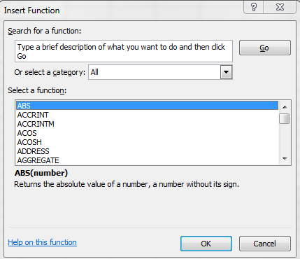
Figure 3.1: Use the insert function button to insert a function in Excel.
If you select the function called SUM, a new dialogue box opens, where you type in the arguments. For example, if cell A1 had the number 2 in it, and cell B1 had the number 3 in it, you could add the two together by “passing” the values stored in cells A1 and B1 to the function:
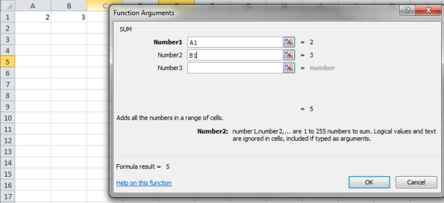
Figure 3.2: Passing arguments to a function in Excel.
Alternatively, you may have used this function directly by typing in the formula bar:
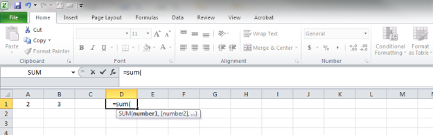
Figure 3.3: Typing a function in Excel’s formula bar.
Both examples show how you would use Excel to add the contents of cell A1 to the contents of cell B1. In both cases, you would fill in the arguments as shown, or type this equation into a blank cell: =SUM(A1, B1). The function’s name is SUM, and in this example there are two arguments: cells A1 and B1. In the code, note that the different arguments are separated by a comma.
This code sends the contents of cells A1 and B1 to the SUM function, which adds them together and returns the result. As such, we say that argument values are “fed” or “passed” into the function, and the function then uses those inputs to do something else.
R functions work the same way. The function name is typed first, followed by arguments within parentheses, where different arguments are separated by commas. If you see a parenthesis in some R code, there’s more than a good chance that it is either opening or closing a function.
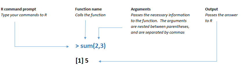
Figure 3.4: A function in R has a specific structure.
Open a new R script file and save it as chapter3.R your R_for_Fledglings directory. Use this script for all of this chapter’s work.
Type sqrt(100) in your script, and submit it. Here, the function name is sqrt, and we are passing a single argument to this function, the number 100. As you have guessed, R will return the square root of 100.
## [1] 10What R actually returned is [1] 10. The number 10 is obviously the answer we are looking for, but what is the [1]? In this example, R computes the square root of 10 and stores the result in an object, and returns the first element of that object. We’ll overview R’s objects in the next chapter.
In order for an R function to be executed, you need to provide it the arguments it needs. How do you know exactly what arguments are needed? In Excel, you can use the insert function button to open up a dialogue box that walks you through the arguments (or just type the function name and Excel shows the arguments). There is no dialogue box in R, but there are two ways to find the arguments a function is expecting. First, you can use the help function, and pass in the function’s name. For example, type help(sqrt) to run a function called help and pass it the argument sqrt:
RStudio responds to this command by bringing the Help tab in the lower right hand pane into focus, which displays the helpfile for the function, sqrt. Looking through the documentation in the helpfile, we see several sections:
- The section, “Description”, provides a short description of the
sqrtfunction: “…computes the principle square root of x”.
- The section called “Usage” provides the text required to call the function, and provides some typical ways of using the function. Here it says “sqrt(x)”. You may also see examples of the function in action in the “Examples” section of the helpfile.
- Under the section called “Arguments”, we see that this function has one argument that is named “x”.
- There are other sections too, which we’ll learn about in future chapters.
You may have noticed the function abs is included in the sqrt helpfile. What’s it doing there? The abs and sqrt functions are grouped together as ‘Miscellaneous Mathematical Functions’ in R’s helpfile system.
You can also find the arguments of a function by using the args function, where you pass in the function’s name:
## function (x)
## NULL
After the word function, you’ll see the names of this function’s arguments within a set of parentheses. Here, there is one argument, “x”. Of course, the letter “x” is not a number and you can’t take the square root of the letter “x”. The “x” is just the name of the argument . . . you assign a value for x, and pass this to the function: sqrt(100). To make it more clear from a coding perspective, you can include the name of the argument in your code and assign that argument a value, as shown below:
## [1] 10Now we know the name of the function sqrt, the name of the argument (x), and the argument’s value (100). R will execute the function and return the answer, 10.
Now try typing Help(sqrt), with a capital H.
Error: could not find function "Help"What happened? R tells us that it could not find a function called Help. Keep in mind that R is case-sensitive, so “help” is not at all the same thing as “Help”.
Let’s try another function called citation. First, let’s take a look at the helpfile:
After you’ve read through the help file, run the function. Type citation() after the prompt, and then press Enter or Return.
##
## To cite R in publications use:
##
##   R Core Team (2020). R: A language and environment for statistical computing. R Foundation for Statistical Computing, Vienna,
##   Austria. URL https://www.R-project.org/.
##
## A BibTeX entry for LaTeX users is
##
##   @Manual{,
##     title = {R: A Language and Environment for Statistical Computing},
##     author = {{R Core Team}},
##     organization = {R Foundation for Statistical Computing},
##     address = {Vienna, Austria},
##     year = {2020},
##     url = {https://www.R-project.org/},
##   }
##
## We have invested a lot of time and effort in creating R, please cite it when using it for data analysis. See also
## 'citation("pkgname")' for citing R packages.
You should see that R returns information to the console that provides information on how to properly cite R.
When you type citation(), you are invoking the function called citation and are sending NO arguments inside the parentheses, which looks like this: ( ). Since you didn’t specify an argument, R will use the function’s default values and return information on how to cite the R base package. The args function can be used to find out what the default values are:
## function (package = "base", lib.loc = NULL, auto = NULL)
## NULL
Here, you see that the citation function has three arguments: package, lib.loc, and auto. Notice that the argument names can contain a period, and that each argument name is separated by a comma. The default value for the package argument has been set to “base”, as indicated by package = “base” above. So, if you do not specify a package name, the function will use the default and return the citation for R’s base package. You could get the same result by typing citation(package = “base”), which makes it crystal clear that you are invoking a function called citation, and assigning the argument named package a value of “base” . . . R will provide the citation for the base package.
The other two arguments (lib.loc and auto) have default values set to NULL. This means that these arguments are not required. Because the arguments have a default value or are not required, we can get away with typing citation() and still get a result.
Now let’s try a function that has two arguments. This time, we’ll use a function that lets us round a decimal number. In the sixth grade we learned that the value for pi is indeterminate; there are an apparently infinite number of decimal values. In R we can quickly call the number pi with two simple letters:
## [1] 3.141593If we want to round this value to the more commonly used value of 3.14, we use the round function, which has two arguments.
First, let’s consult the help file.
Now let’s use the args function to look at the arguments directly.
## function (x, digits = 0)
## NULL
You can see that the two arguments to round function are called x (the value to round) and digits (the number of digits we want to see to the right of the decimal point). Recall that the description of these arguments can be found in the help tab associated with this function (i.e. by typing help(round)). So to convert pi to 3.14, we will round to two decimal points like this:
## [1] 3.14The args function also showed us that that the default for the digits argument is 0, so if we do not specify a value for digits, the function will round to 0 places. The lesson here is to always, always check the default values.
## [1] 3You aren’t required to type in the argument names. As long as you enter the arguments in their proper order, there is no need to name them. For example, you could have entered:
## [1] 3.14This works because the arguments are provided in the proper order that the function expects them. If you don’t name them and mix up the order, the function will either return an error (which indicates a problem with your coding) or will return an incorrect value. Try it:
## [1] 2In this example, R interprets your command as “round the integer 2 to 3.14 decimal places”, and it returns the number 2 – which is not what you really wanted. An important lesson here is that R will not always return an error, and if you are not careful in your coding you could end up with unintentional mistakes and merrily continue unaware of your error.
Because of this, throughout this book we’ll be adding in argument names for functions with more than one argument because we think it makes coding more clear. This is useful especially if you will be sharing your code with others, or if you will be reusing pieces of code at a later time and need to jar your memory about what a particular function is doing. We will also attempt to follow additional rules in the tidyverse style guide to keep our code clean.
RStudio provides a tremendous helper for entering arguments of a function in a script. When you type in the function’s name and then open the first parenthesis, press the tab key – RStudio will display a small pop-up that allows you to select an argument and type in a value.
Figure 3.5: RStudio’s tab helper is super useful!
If you select an argument, then press tab again, the argument name will be inserted into your code automatically and you can type in the value for the argument you need. Or, if a list of argument values is presented, you can select the option you want and press tab again and the argument value will be auto-inserted. As you enter commas after an argument, press tab again and you can work your way through the various arguments quickly. This tab trick works for digging into objects too!
Now let’s try a function with three arguments. We’ll use the function, seq, to create a sequence of numbers from -9 to +9. First, as always, take a look at the helpfile. (You were just about to do that without a prompt, right?)
The Description section indicates that the function is used to generate regular sequences (i.e., sequences that are predictable). Under the Arguments section, you see five arguments listed:
- …
- from, to
- by
- length.out
- along.with
Under the Details section of the helpfile, you can see different examples of how this function is most often used. One of these indicates seq(from, to, by =). In this form, the function uses three of the arguments: from, to, and by. And in the Examples section, several different examples are provided, including seq(1, 9, by = 2). This looks similar to what we need for creating our sequence from -9 to +9 by units of 1. Let’s try it, but add in the argument names for clarity.
## [1] -9 -8 -7 -6 -5 -4 -3 -2 -1 0 1 2 3 4 5 6 7 8 9As we’ve seen, not all arguments are required. For instance, in executing this code, we did not use the length.out or the along.with arguments. Thorough reading of the function’s help file, or liberal use of the args function, will reveal which arguments are required versus which are optional.
The seq function brings up another important thing about functions. Several functions have a “dots” argument, which looks like three periods or dots (known in formal grammar as an ellipsis), and is described in the helpfile as “arguments passed to or from methods”. We’ll dig into the dots arguments later in the book (when we need to use them).
We’ve mentioned that a function is a chunk of code that gives R some instructions to carry out. R is open source, which means that you can actually see the code for a function if you wish to inspect it. Just type in the name of the function, and R will provide the code that it executes when this function is called. Let’s scan the code for the citation function (no parentheses):
## function (package = "base", lib.loc = NULL, auto = NULL)
## {
##     if (!is.null(auto) && !is.logical(auto) && !any(is.na(match(c("Package",
##         "Version", "Title"), names(meta <- as.list(auto))))) &&
##         !all(is.na(match(c("Authors@R", "Author"), names(meta))))) {
##         auto_was_meta <- TRUE
##         package <- meta$Package
##     }
##     else {
##         auto_was_meta <- FALSE
##         dir <- system.file(package = package, lib.loc = lib.loc)
##         if (dir == "")
##             stop(packageNotFoundError(package, lib.loc, sys.call()))
##         meta <- packageDescription(pkg = package, lib.loc = dirname(dir))
##         citfile <- file.path(dir, "CITATION")
##         test <- file_test("-f", citfile)
##         if (!test) {
##             citfile <- file.path(dir, "inst", "CITATION")
##             test <- file_test("-f", citfile)
##         }
##         if (is.null(auto))
##             auto <- !test
##         if (!auto) {
##             return(readCitationFile(citfile, meta))
##         }
##     }
##     if ((!is.null(meta$Priority)) && (meta$Priority == "base")) {
##         cit <- citation("base", auto = FALSE)
##         attr(cit, "mheader")[1L] <- paste0("The ", sQuote(package),
##             " package is part of R.  ", attr(cit, "mheader")[1L])
##         return(.citation(cit, package))
##     }
##     year <- sub("-.*", "", meta$`Date/Publication`)
##     if (!length(year)) {
##         if (is.null(meta$Date)) {
##             warning(gettextf("no date field in DESCRIPTION file of package %s",
##                 sQuote(package)), domain = NA)
##         }
##         else {
##             date <- trimws(as.vector(meta$Date))[1L]
##             date <- strptime(date, "%Y-%m-%d", tz = "GMT")
##             if (!is.na(date))
##                 year <- format(date, "%Y")
##         }
##     }
##     if (!length(year)) {
##         date <- as.POSIXlt(sub(";.*", "", trimws(meta$Packaged)[1L]))
##         if (!is.na(date))
##             year <- format(date, "%Y")
##     }
##     if (!length(year)) {
##         warning(gettextf("could not determine year for %s from package DESCRIPTION file",
##             sQuote(package)), domain = NA)
##         year <- NA_character_
##     }
##     author <- meta$`Authors@R`
##     if (length(author)) {
##         aar <- .read_authors_at_R_field(author)
##         author <- Filter(function(e) {
##             !(is.null(e$given) && is.null(e$family)) && !is.na(match("aut",
##                 e$role))
##         }, aar)
##         if (!length(author))
##             author <- Filter(function(e) {
##                 !(is.null(e$given) && is.null(e$family)) && !is.na(match("cre",
##                   e$role))
##             }, aar)
##     }
##     if (length(author)) {
##         has_authors_at_R_field <- TRUE
##     }
##     else {
##         has_authors_at_R_field <- FALSE
##         author <- as.personList(meta$Author)
##     }
##     z <- list(title = paste0(package, ": ", meta$Title), author = author,
##         year = year, note = paste("R package version", meta$Version))
##     if (identical(meta$Repository, "CRAN"))
##         z$url <- sprintf("https://CRAN.R-project.org/package=%s",
##             package)
##     if (identical(meta$Repository, "R-Forge")) {
##         z$url <- if (!is.null(rfp <- meta$"Repository/R-Forge/Project"))
##             sprintf("https://R-Forge.R-project.org/projects/%s/",
##                 rfp)
##         else "https://R-Forge.R-project.org/"
##         if (!is.null(rfr <- meta$"Repository/R-Forge/Revision"))
##             z$note <- paste(z$note, rfr, sep = "/r")
##     }
##     if (!length(z$url) && !is.null(url <- meta$URL)) {
##         if (grepl("[, ]", url))
##             z$note <- url
##         else z$url <- url
##     }
##     header <- if (!auto_was_meta) {
##         gettextf("To cite package %s in publications use:", sQuote(package))
##     }
##     else NULL
##     footer <- if (!has_authors_at_R_field && !auto_was_meta) {
##         gettextf("ATTENTION: This citation information has been auto-generated from the package DESCRIPTION file and may need manual editing, see %s.",
##             sQuote("help(\"citation\")"))
##     }
##     else NULL
##     author <- format(z$author, include = c("given", "family"))
##     if (length(author) > 1L)
##         author <- paste(paste(head(author, -1L), collapse = ", "),
##             tail(author, 1L), sep = " and ")
##     rval <- bibentry(bibtype = "Manual", textVersion = paste0(author,
##         " (", z$year, "). ", z$title, ". ", z$note, ". ", z$url),
##         header = header, footer = footer, other = z)
##     .citation(rval, package)
## }
## <bytecode: 0x000000002a03f788>
## <environment: namespace:utils>
Yowza! You can see that there is a lot going on behind the scenes when we use the citation function. Don’t worry about interpreting this code. The main point is that you can call up the function’s code by just typing in the function name.
Exercise 1:
- Look at the helpfile for the following functions:
- rep
- log
- floor
- Compare the helpfile for
repwith the helpfile forreplicate. Use the helpfile to determine when you would userepand contrast it with when you would usereplicate.
3.1 Nested Functions
Let’s return to the sqrt function helpfile and take a look at the section called “Examples”.
The Examples section of a helpfile can be helpful, so don’t ignore this section. The idea behind the Examples section of a helpfile is to provide example code that shows how the function can be used, starting with the creation of some sample data, and then demonstrating how to use the function on the sample data. You can learn a lot by copying and pasting the code into the Console, and then submitting it. Here, we’ll just copy two lines of code from the sqrt helpfile example and paste it into this chapter’s script:

Figure 3.6: Plot generated from code in R’s helpfile.
In line 1 of this code, we created an object called “xx” which has the integers -9 to 9 in increments of 1. The colon operator (:) is another way of creating a sequence in R. If you want to have a look at xx, just type in xx and send it to the R console. (We will cover objects in great depth in the next chapter.)
Line 2 of this code is typical R helpfile code that nests several functions together in short, concise code. Expert coders try to keep their code as tight as possible . . . for them it is concise, easy to follow, and someone else that uses their code will not have to wade through several lines of code to get to the result. All of this is fine and well . . . as long as you are not a fledgling. If you are a beginner, this code can be daunting. You can make headway if you break the code apart. Remember to look for a function’s opening and closing parentheses, and recall that arguments are always separated by commas. Let’s work through this line of code:
There are three functions in play here. You know the sqrt function, but can you also see the abs function in this code? Let’s find out what this function does:
So the abs function returns the absolute value. How about the plot function? We used the plot function in Chapter 2, but now let’s look for its arguments by calling up the helpfile (the args function isn’t too helpful in this case):
Under the Usage section of the helpfile, we see that plot requires an argument called x, which is a list of values that goes along the x-axis of a plot. For each value of x, the plot function needs a corresponding y value, which is given by the argument called y. An optional argument is called col, which is short for color.
Now that you know what arguments each function needs, let’s look at the sqrt helpfile code once more:
plot(xx, sqrt(abs(xx)), col = “red”)
Here, the plot function’s open parenthesis is right after the word, plot. The close of the plot function is at the very end of the line, after the word “red”. These are highlighted in red, but you can track the location of the “matching” parentheses by clicking immediately after the first opening parenthesis in your script . . . the closing parenthesis for the function should be highlighted. Try it!
We’ve seen that the plot function has several arguments, of which x and y are critical. Because the object xx is listed as the first argument, we can assume that it is the value for plot argument, x (so the numbers -9 to 9 will occupy the x-axis). We can also assume that the second argument of the plot function, y, is specified by the code sqrt(abs(xx)). Another comma is present after this argument, and then we see a third argument for the plot function, col, and that the value for this argument is set to red. Note that adding a space in between arguments is not required by R, but is helpful for visually reading the code . . . much like reading words written this way is easier than readingwordswrittenthisway!
If we include the names of the arguments described in the sqrt helpfile code,
plot(xx, sqrt(abs(xx)), col = “red”) could be written as:
This makes it clear that the x argument for the plot function is xx (a series of numbers from -9 to 9), and the y argument for the plot function is a series that contains values from sqrt(abs(xx)). The final argument for the plot function is col, and its value is set to “red”.
Now let’s focus on the second argument value, which is sqrt(abs(xx)), which sets the y axis for the plot function. What’s going on here? Well, you should recognize the sqrt function, which opens right after the word sqrt and closes after abs(xx). We know the sqrt function has one argument, named x, and we also know that the abs function has just one argument, also named x.
We could rewrite sqrt(abs(xx)) as:
But here is a case where adding the argument name can get a little confusing because the name of the argument x in both functions is similar to the name of our object, xx. Do you agree?
As long as you already understand that the sqrt and abs functions have a single argument, this seems a bit cleaner:
If we were to re-write the sqrt helpfile code so that it included the argument names for the plot function for added clarity, we would type:
Figure 3.7: Plot from R helpfile, with argument names added.
This is an example of three “nested” functions. Hopefully you can see that R will need to execute the inner-most function, abs, before it can execute the sqrt function, and the sqrt function must be executed before the plot function can be executed.
By the way, you’ve probably noticed that all three of the functions have an argument that is called x. Keep in mind that argument names are specific for each function: the argument named x in the plot function is totally different than the argument named x in the sqrt function. This is because the author of each function gets to choose the argument names (as well as the name of the function).
The R helpfiles are loaded with examples that have nested functions. This book is targeting a beginner R audience, and for you beginners out there, it is far, far better to write code in smaller pieces that you completely understand than to write code that you’re not sure what it is doing.
Let’s try to get the same result as the sqrt helpfile code by breaking it down into pieces as we have discussed, knowing that we will be plotting a series of x values against a series of y values in the plot function. First, create an object called xx with the integers -9 to 9 (in order).
# create an object called "xx" from -9 to 9 by increments of 1
xx <- -9:9
# look at the object called "xx"
xx
## [1] -9 -8 -7 -6 -5 -4 -3 -2 -1 0 1 2 3 4 5 6 7 8 9These numbers make up our “x” values for the plot function. (Incidentally, objects like xx that contain a single series of numbers are called vectors. These will be described in Chapter 4.)
For the “y” values, we take the absolute value of xx with the abs function and send them to an object called yy.
# take the absolute value for each element of xx, and store the result in a new object called yy.
yy  <- abs(xx)

# look at the object called "yy"
yy
## [1] 9 8 7 6 5 4 3 2 1 0 1 2 3 4 5 6 7 8 9Notice that the abs function worked on each and every number within the object, xx, a process known as “vectorization.” So our new object, yy, is a vector of numbers that are all non-negative numbers.
Next we take the square root of each value in the object yy…these represent our “y” series for plotting.
# take the square root of each value stored in the object, yy.
# replace the original object called "yy" with this new result
yy  <- sqrt(yy)

# look at the object called "yy" and notice that it now has different values
yy
## [1] 3.000000 2.828427 2.645751 2.449490 2.236068 2.000000 1.732051 1.414214 1.000000 0.000000 1.000000 1.414214 1.732051 2.000000 2.236068 2.449490
## [17] 2.645751 2.828427 3.000000Finally, we plot all of the x’s against all of the y’s with the plot function, and use red as the col argument so that our datapoints are shaded in red:
Figure 3.8: Plot from re-imagined R helpfile.
This little exercise hopefully re-enforces a key concept R coding: if it takes a few more lines of code to get the result you need (and most importantly a result that you understand), by all means use more lines of code.
Exercise 2:
Compute the square root of pi, round it to four decimal points, and assign the output to an object. Be sure to choose a descriptive name!
Take the natural log of your number, and then truncate the result (heh, heh, heh . . . you’ll have to find these functions).
Answers to all exercises are posted at the end of the chapter.
3.2 Operator Functions
We’ve indicated that functions have names, followed by arguments that are enclosed within a set of parentheses. There are a few functions that you’ll use repeatedly that do not require a name, but rest assured they are still functions. Here are a few examples:
- + (addition)
- - (subtraction)
- / (division)
- ^ (exponentiation)
- %% (modulus)
- %/% (integer division)
If you search on these in the helpfile with help(“+”), you’ll see that R describes these as “unary and binary operators [that] perform arithmetic on numeric or complex vectors . . .”. These operators are what you’d expect in a calculator.
Here are some more operators, which won’t be found on a calculator:
- : (the colon operator, used to generate regular sequences, as in “x <- -9:9”)
- :: (the double colon operator, used for specifying a package name and function)
- ~ (the tilde operator, used to separate the left and right hand side of a model formula)
Just like nested functions call for an ordering of execution, these operators have an order of operation, and follow PEMDAS, which follows the mnemonic “Please Excuse My Dear Aunt Sally” we learned in 5th grade. What this actually stands for is Parentheses, first, followed by Exponents, followed by Multiplication and Division (left to right), followed by Addition and Subtraction. But R has more operators and thus must be expanded. For example, the colon operator is evaluated before PEMDAS.
In addition, another function we’ll use repeatedly is the extractor function, which looks like this [ ] or this [[ ]]. To see the helpfile on this function, use the following:
The R helpfile tells us that these are “operators acting on vectors, matrices, arrays and lists to extract or replace parts.” We’ll work with these extensively in the next chapter.
3.3 Generic Functions
Some functions are known as generic functions. The print function that we touched on briefly in the last chapter is an example of a generic function. We won’t go into many details here, but generally speaking, a generic function like print has alternative forms, or “methods” of execution. For example, if you look at the print helpfile, you’ll see a reference to the functions, print.table, print.factor, and print.default. The function name is still print, but the method that R uses to print is defined by the method name (after the period). For example, if you use the print function and ask R to print an object of class “table”, R will actually use the print.table function behind the scenes. In most cases, you don’t need to worry about what is happening behind the scenes . . . just use print and R will do the rest.
3.4 Packages
In Chapter 1, you saw that R is a both a computation platform and an interactive language. The R platform consists of about 30 core packages, each of which contains functions for your use. For example, the sqrt, abs, and plot functions that we have used so far are included in one of the 30 base packages. Many (but not all) of the base packages are automatically loaded when you start R, and they provide the foundation that interprets each function we type for computing or plotting.
So, how do you find which packages R is using? There are two ways. First, click on the Environment tab in upper right pane of RStudio, and then select the drop-down arrow by the words Global Environment. We’ll touch on the topic of environments in the next chapter, but for now, you should see a list of packages that were attached by default when you started R.
Figure 3.9: Packages that are loaded when you start an R session.
Clicking one of these will open a list of functions or objects associated with the selected package. For example, click on package:datasets and you’ll see the many datasets (objects) that come with R (this image is in Grid View as opposed to List View; look for the toggle in the upper right hand corner of the Environment tab). Many helpfile examples in R take advantage of these datasets to demonstrate the use of a function.
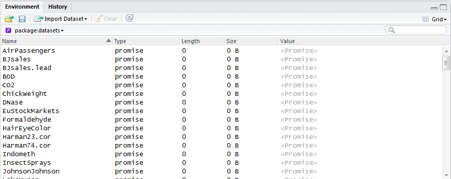
Figure 3.10: R comes with many built-in datasets in the datasets package.
In case you were wondering, a promise is a special type of object in R that takes on ‘life’ when it is called. For example, notice that the dataset called ChickWeight has a value of <Promise> in the screen shot above. We can call this dataset by just typing its name. Here, we’ve used the head function to look at the first 10 records only.
##    weight Time Chick Diet
## 1      42    0     1    1
## 2      51    2     1    1
## 3      59    4     1    1
## 4      64    6     1    1
## 5      76    8     1    1
## 6      93   10     1    1
## 7     106   12     1    1
## 8     125   14     1    1
## 9     149   16     1    1
## 10    171   18     1    1
Now if we look at the package: datasets in the Environment tab, we see that this dataset is 21.4 KB in size, contains 4 variables (columns) and 578 observations (rows).
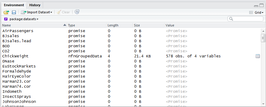
Figure 3.11: The chickweights dataset is no longer a promise.
The second way to see which packages are loaded into your R session is to use RStudio’s Package tab. Click on the Packages tab in the lower right pane of RStudio, and you’ll see a list of some of the packages that were installed when you installed R. Those that are loaded into your R session should have a check-mark near them. (Your list might look slightly different than ours).
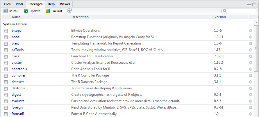
Figure 3.12: The Packages pane in R.
You can see a list of package names, each with a short package description and their installed version. We’ll return to this tab in a few minutes.
A third way to see which packages are loaded is to use the sessionInfo function, with no arguments:
## R version 4.0.2 (2020-06-22)
## Platform: x86_64-w64-mingw32/x64 (64-bit)
## Running under: Windows 10 x64 (build 17134)
##
## Matrix products: default
##
## locale:
## [1] LC_COLLATE=English_United States.1252  LC_CTYPE=English_United States.1252    LC_MONETARY=English_United States.1252
## [4] LC_NUMERIC=C                           LC_TIME=English_United States.1252
##
## attached base packages:
## [1] stats     graphics  grDevices utils     datasets  methods   base
##
## other attached packages:
##  [1] roxygen2_7.1.1       devtools_2.3.0       usethis_1.6.1        rgdal_1.5-16         sp_1.4-2             dplyr_1.0.0
##  [7] tidyr_1.1.0          ggplot2_3.3.2        lubridate_1.7.9      readxl_1.3.1         clipr_0.7.0          knitr_1.30
## [13] knitcitations_1.0.10 bookdown_0.21        rmarkdown_2.6
##
## loaded via a namespace (and not attached):
##  [1] Rcpp_1.0.5        lattice_0.20-41   prettyunits_1.1.1 ps_1.4.0          assertthat_0.2.1  rprojroot_1.3-2   digest_0.6.25     R6_2.4.1
##  [9] cellranger_1.1.0  plyr_1.8.6        backports_1.1.10  evaluate_0.14     highr_0.8         httr_1.4.2        pillar_1.4.6      rlang_0.4.10
## [17] rstudioapi_0.11   callr_3.5.1       desc_1.2.0        RefManageR_1.2.12 stringr_1.4.0     munsell_0.5.0     compiler_4.0.2    xfun_0.20
## [25] pkgconfig_2.0.3   pkgbuild_1.1.0    htmltools_0.5.0   tidyselect_1.1.0  tibble_3.0.3      crayon_1.3.4      withr_2.3.0       grid_4.0.2
## [33] jsonlite_1.7.1    gtable_0.3.0      lifecycle_0.2.0   magrittr_1.5      scales_1.1.1      bibtex_0.4.2.2    cli_2.3.0         stringi_1.5.3
## [41] fs_1.4.2          remotes_2.2.0     testthat_3.0.1    xml2_1.3.2        ellipsis_0.3.1    vctrs_0.3.4       generics_0.0.2    tools_4.0.2
## [49] glue_1.4.2        purrr_0.3.4       processx_3.4.4    pkgload_1.1.0     yaml_2.2.1        colorspace_1.4-1  sessioninfo_1.1.1 memoise_1.1.0
The function returns information about what version of R you are using, what platform you are running R on, and other information. The section “attached base packages” are those that you saw in the environment dropdown we looked at previously. The results may also display “other attached packages”, and an additional section called “loaded via a namespace (and not attached)”. In the latter case, these are packages that R can access, but you cannot access the functions until you load them first with the library function. We’ll get to this function in a few minutes. The packages shown above include some of those we needed to write this book.
3.4.1 Packages on the CRAN repository
In addition to R base packages, the CRAN-R website lists an additional 16000+ contributed packages which can be downloaded and installed to extend the number of functions at your disposal. Think of these packages as “add-ins” or “extensions”. Each R user can install as many of these “add-in” packages as they wish. If R incorporated every package into the core program it would become too bulky, and most packages are too specialized for general use. Thus, this sort of a la carte add-in approach is much more efficient for users.
Exercise 3:
- Go to the CRAN package repository, and examine
the list of available packages. These are conveniently sorted by date of publication or by name.
Each package is given a very brief description.
- Locate the names of two or three packages that you think may help you in your own work.
- Click on one of the package names of interest, and examine the package description page. Do NOT install any packages at this time.
As we mentioned, packages can be hosted in a variety of locations, but the CRAN repository is “package central”. There are several sections on the package’s website page worth noting. In the image below, we selected a package named “unmarked”, which is a set of functions for hierarchical modeling of animal abundance or occupancy from unmarked (and marked) animals.
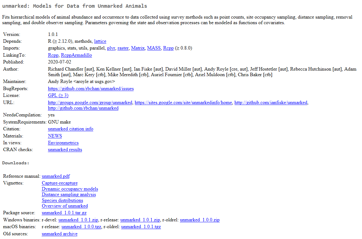
Figure 3.13: The R package, unmarked.
As you can see, this page gives a lot of information, including version information. A few things to notice:
- “Depends” and “Imports”. These indicate packages that this package uses. For example, when the authors of this package created some functions, they may have used functions from other packages in their code. Fortunately, the packages that unmarked needs will also be installed automatically when you install unmarked. The difference between “depends” and “imports” is described in CRAN’s documentation for writing extensions:
Packages whose namespace only is needed to load the package using library(pkgname) must be listed in the “Imports” field and not in the “Depends” field. Packages that need to be attached to successfully load the package using library(pkgname) must be listed in the “Depends” field, only. Read this old but informative blog-posting if you’d like to dive deeper.
- “Author” provides the list of people who wrote the functions of the package. Remember, a package is only as good as its author(s).
- “Maintainer” is the name of the person who is responsible for keeping the code.
- “BugReports” identifies where to report any bugs you may find. A “bug” here is not an insect; it is a coding mistake. If this section is missing, submit your bug report to the package maintainer.
- “URL” provides website addresses of interest. For instance, the authors of this package maintain an active Google Group.
- “Citation” indicates how the package should be cited.
In the Downloads section, you’ll find:
- “Reference manual” - a link to a pdf file that is the documentation for the package. When you use the
helpfunction, you are dipping into that manual, so to speak. Click on the reference manual for your selected package, and you should see the same basic information as the package “home page”, followed by a list of functions in alphabetical order. Clicking on a function name will bring up the same information you’ve seen by using thehelpfunction.
- “Vignettes” - additional documentation on how to use the package. These are usually very, very helpful when you are using a package for the first time. While the “reference manual” is a list of functions, the “vignettes” are more or less tutorials on how to use the package in a reader-friendly format.
- The Package source, MacOS X binary, and Windows binary are the packages themselves, which includes the code for several functions, along with the helpfiles. Which package you download depends on which operating system you use.
We’ll be building a small package in Chapter 10, so you’ll see first hand how a package is created.
3.4.2 Finding Packages on the Internet
As we mentioned in Chapter 1, packages can be hosted on Comprehensive R Archive Network (CRAN), GitHub, R-Forge, and many other locations. Our own packages are maintained on a USGS GitLab site. With thousands of packages available, there’s a good chance that a package has been developed for the task you need. Oftentimes you can find this with a simple Google search. Sometimes it is useful to add the letter “R” and the word “CRAN” to your search string.
Exercise 4:
Use your favorite search engine and see if you can find packages related to the following topics (again, do not install any packages at this time):
- ARC GIS shapefiles
- Working with dates and times in R
- Working with graphics in R
- Connecting to an Excel file
A website that you might want to bookmark is called R Documentation, which searches all packages listed in Cran R, Bioconductor, and GitHub. You can also use a a variety of R search engines. Check these out!
3.4.3 Installing Packages
When you install a package from CRAN, R will dial into a CRAN server, download one or more specified packages, and then extract and install them onto your computer for you. There are many R users across the globe, so to ensure that packages are always available, R uses a network of “mirrors”, which are servers with identical content. Users can choose the nearest mirror, or the mirror with the least download-time, or even the mirror that synchronizes with the main CRAN server most frequently. RStudio automatically selects the mirror for you, but you can set your own mirror by choosing Tools | Global Options | Packages, and then clicking on the Primary CRAN repository option.
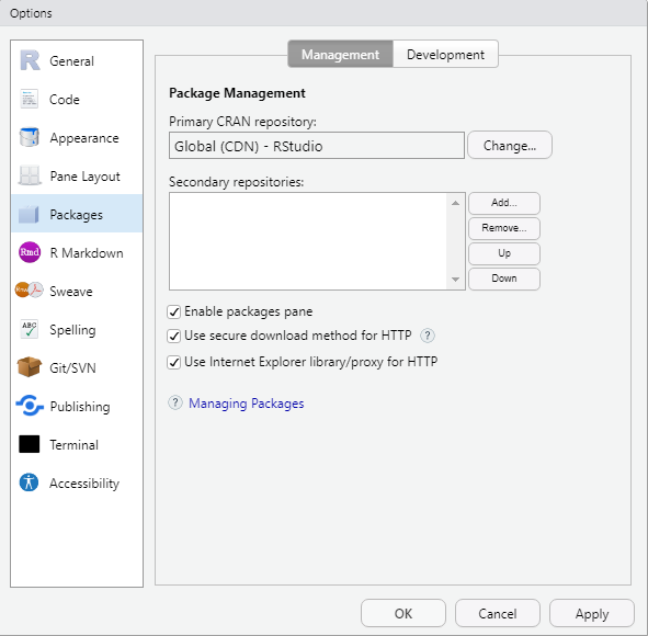
Figure 3.14: Package options.
You can install a package in one of three ways (which we will do in a few minutes - read this first and hold your horses until we specifically tell you to install a package).
First, to download a package within RStudio, you can go to Tools | Install Packages, or click on the small Install Packages button in the Package tab, which looks like this: 
Either of these approaches will display the following dialogue box:
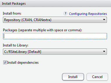
Figure 3.15: Install package dialogue box.
In the dialogue box, you can type in the package name (which is case sensitive), or type in multiple package names each separated by a space or comma. Notice that the “Install dependencies” checkbox is checked by default.
A very important input of the dialogue box is labeled “Install to Library”. When you install your first package, R will ask you if you want to install this package to your site library (also called a user library), and it will recommend a location somewhere on your computer (more on this very important topic in a minute). All subsequent packages you install will be directed to your site library.
Second, we can also install a package via the R console using the function install.packages. For example, if there was a package called “fledglings” , you could install it with the command:
# Notice that package names here are characters and must be quoted
install.packages(pkgs = "fledglings")
Third, to download a package outside of CRAN, you can download the package as a .zip (Windows users) or tar.gz file (Mac or Linux users). Then, in RStudio’s Install Package pane, click the dropdown arrow in the “Install from” option, and select "Package Archive (.zip; .tar.gz). Then navigate to your downloaded file:
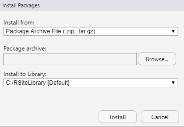
Figure 3.16: Install package from a local source.
These button clicks are actually running the install.packages function, and pointing to a locally stored package file. It’s worth your time to read through this function’s helpfile.
We listed three ways to install packages above, in the order you are most likely to employ them. The first way is the easiest, and the RStudio mirror is a good default choice for most users because it should offer relatively stable download speeds for users across the globe. If you find your downloads are slow you may select a different, nearby mirror.
The second method and third methods are the most flexible as you have access to all of the arguments in the install.packages function.
Before we actually install any packages, it’s very important that you understand the concept of ‘libraries’, so we’ll turn to that topic now, and then install a few packages soon thereafter.
3.4.4 Your R Library
When you download R, the core packages are stored in a library, which is a directory on your computer. So, how exactly do you find your library? Use the library command, and send no arguments:
RStudio will display a new tab in the Files pane, and this tab will list all of the packages associated with R. You may see only one section, which might look something like Packages in library C:/Program Files/R/R-4.0.2/library. If you are a PC user and installed a package already, you may see two sections (Mac users will normally see only one library).
Another way of finding the path to your libraries is to use the .libPaths function:
## [1] "C:/RSiteLibrary" "C:/Program Files/R/R-4.0.2/library"Here, you can see that we have two libraries (again, you may have only one). And again, we are on a PC; your results may look different.
The R “base” packages, which are stored in your Programs directory under R. Ours is stored at C:/Program Files/R/R-4.0.2/library. R created this library when we installed R. Here you can find the packages we looked at in the Environment tab, such as base, graphics, datasets, and others. Only R’s core packages should be in this library…don’t touch it. The library that core R packages are stored in is write-protected by default, so unless you are truly stubborn you will not be able to store your personal packages there.
The library where R installs all add-on packages, the “user” library or “site” library. Ours happens to be stored at C:/RSiteLibrary. Any new packages that we choose to install would be added to this library.
If you are on a Mac, you probably have only one library, and the .libPaths() call will return something like this:
/Library/Frameworks/R.framework/Versions/4.0/Resources/libraryWhen you click on the Packages pane in RStudio, the list reflects packages from all libraries. The separation of the “core library” and “site/user library” is by design; your library will be better organized and you will be able to add and delete packages at will if you have a site library that is specific to the current user-account on your computer, and to which you have write-permission. The site library R creates can be used for a long time, as long as the updates to R are all minor (e.g. all R versions 3.0.0 - 3.9.9 can use the same site library). However, if there are major updates to R (e.g., R version 4.0 and up), you will need to re-create your site library if you are a Windows user.
If you haven’t installed a package yet, and click on Install button in RStudio (or use some other option), you’ll see that R will try to create a site library for you if you are on a PC. We work at a university setting, and R wanted to add a site library on the University of Vermont network. But we’ve learned, after many hours of frustration, that it is easiest to keep your site library off the network, say, in a folder on your C drive. In later chapters, we will be creating a package and you will need to be able to write to your site library. If you work on a network and are a PC user, we strongly suggest that you read the section below!
If you want to establish your own site library, say, on your C drive (or anywhere off the network) in a folder called RSiteLibrary, you can do so and then tell R where to find it. Here are the steps for PC users:
- Create a folder on your C drive called RSiteLibrary.
- Navigate to the file called Rprofile.site. This file is most likely stored in etc folder in the path: Program Files | R | R-4.x | etc. To verify this, use the
R.homefunction with no arguments:
## [1] "C:/PROGRA~1/R/R-40~1.2"The file Rprofile.site may be write-protected or indicate that access is denied. In this case, you should copy it over to your desktop, and then open it with RStudio or some other text editor. Our file looks like this (note that many of these options are commented out):
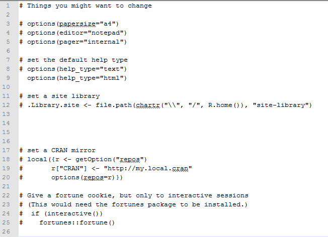
Figure 3.17: The Rprofile.site file.
- Add the following line to the end of the script: .libPaths(“C:/RSiteLibrary”) Make sure that the quotes match with the quote style in the document (e.g., if your quotes are tilted and the quotes in Rprofile.site are untilted, make your quotes untilted.)
- Save the file. Then copy it back to the folder where you found it. You may get a message saying that you need administrator permissions . . . click “Continue” if you can.
- Now restart R, and call .libPaths again.
[1] "C:/RSiteLibrary" "C:/Program Files/R/R-4.0.2/library"Hopefully you now see two libraries listed. Of course, you can elect to let R create a site library for you and use the defaults. Just be prepared for potential frustrations if you live on a network. Regardless, just being aware that there are multiple libraries is worthwhile.
Mac users, read this post, section 3.4 to learn about how your R libraries are stored on your Mac.
The Package Installer performs installation to either place depending on the installation target setting. The default for an admin users is to install packages system-wide, whereas the default for regular users is their personal library tree.
Finally, we are ready to install some packages. We’ll start by installing the package rgdal, a geospatial package that we’ll use in future chapters.
Exercise 5:
- Find the package rgdal on the CRAN package repository, and read through the package “home page”.
- Install the package rgdal on your machine using one of the three methods described.
- Press the “refresh” button in the Package Pane (to the right of Check for updates), and look for your package.
Hopefully, that went well. It might be instructive to actually look at the files you just added to your site library.
Exercise 6:
- Locate where your site library is stored on your computer (e.g. C:/RSiteLibrary).
- Navigate to the rgdal folder within your site library.
- Peer into the package’s folders, and look at the contents. Don’t edit anything though!
All of these files were created by the authors of the package, rgdal. In chapter 10, we’ll show you how to create a simple package, which should take some of the mystery away.
3.4.5 Updating Packages
Packages may be updated frequently, and R itself is updated twice a year. To make sure that you are running the most recent versions, in RStudio go to Tools| Check for Package Updates, or click on the Check for Updates button in the Packages pane 
You can also use the packageStatus and update.packages functions to check on the status update your packages from the console. This is preferable if you wish to use any of the arguments to the update.packages function.
3.4.6 Using a Package in R
Downloading packages is something you typically only need to do once (until a major R version is introduced). To actually use a package in an R session, you need to call them up from your package library. This is done with the library function, where the package name is entered as the argument to the library function:
This particular package has a fairly lengthy start-up message, which you should read particularly if this is your first use. To avoid these messages in the future, you could nest the library function call within the function suppressPackageStartupMessages:
Think of your site/user library like your local public library…you can “check out” and “return” books. When you start R, the base library is loaded, but to use functions within a package in your library you must check them out (attach them) with the library function.
Another way to “check out” a package is by clicking the check-box in the Packages pane. You’ll see that R Studio has sent the library function to the R console and executed it.
An important change takes place in R when you load a package. Take a look at what happens in the Environment tab. Click on the drop-down arrow called Global Environment, and then look for the rgdal option:
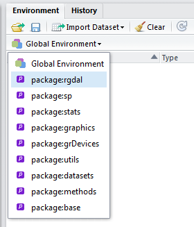
Figure 3.18: The rgdal environment.
When you select the rgdal environment, you are shown all of the functions within this package:
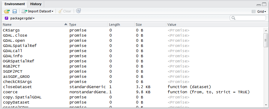
Figure 3.19: The rgdal functions in the rgdal environment.
The collection of functions within a package, then, are stored in a unique environment when it is loaded.
To remove (unload) the library from your environment, uncheck the package in the Packages pane, or use the detach function. You’ll see that when you uncheck the box, RStudio will send the following code to your console:
This action removes (detaches) the package environment from R.
3.4.7 Function Names from Different Packages
Occasionally, authors of one package will use the same function names as authors from another package. When this happens, R will let you know that the function from one package is “masked” by a function from the other package. For example, suppose you load a package called species that contains a function called bears (which retrieves taxonomic characteristics of black bears), and then load a different package called NFLteams that has a function called bears (which retrieves the NFL roster for the Chicago Bears).
In this case, the species version of the bears function will be masked by the NFLteams version (because the NFLteams version was more recently loaded).
To get around that issue, enter
species::bears when you want to run the bears function from the species package, and enter
NFLteams::bears when you want to run the bears function from the NFLteams package.
In this example, we are pointing R to the environment (before the ::), followed by the function within the specified environment. With new packages coming out daily, it’s a good habit to use this convention in your code to avoid collisions!
3.5 Summary
That ends a short, but important introduction to functions. It’s helpful to remember that everything that R does is done via a function. We’ve learned that functions have arguments, some of which contain defaults and some of which may be optional. We’ve stressed that the helpfile and args function are invaluable tools for learning how to use a function. We’ve discussed ‘contributed packages’ as a means of adding on new functionality to your R base program. And we’ve discussed the all-important concept of libraries. We’ll be building on this material in our next chapter, which focuses on objects.
3.6 Answers to Exercises
Exercise 1:
- Look at the helpfile for the following functions:
- rep
- log
- floor
Compare the helpfile for
repwith the helpfile forreplicate. Use the helpfile to determine when you would userepand contrast it with when you would usereplicate.
The rep function is used to repeat an object a certain number of times. The replicate function “is a wrapper for the common use of the function sapply for repeated evaluation of an expression (which will usually involve random number generation).” We will learn about the sapply function in future chapters.
Exercise 2:
- Compute the square root of pi, round it to four decimal points, and assign the output to an object. Be sure to choose a descriptive name!
- Take the natural log of your number, and then truncate the result (heh, heh, heh.you’ll have to find these functions).
# square root of pi
answer  <- sqrt(pi)
# round the answer to 4 digits
answer  <-  round(x = answer, digits = 4)
# take the natural log of the number
answer  <- log(answer)
# truncate result
answer <- trunc(answer)

# all in one step with super nesting!
answer  <- trunc(log(round(x = sqrt(pi), digits = 4)))
Exercise 3
- Go to the CRAN package repository, and examine
the list of available packages. These are conveniently sorted by date of publication or by name.
Each package is given a very brief description.
- Locate the names of two or three packages that you think may help you in your own work.
- Click on one of the package names of interest, and examine the package description page.
Well, what did you find?
There really are no right or wrong answers here, but we hope you found some packages that may assist you with your work.
Exercise 4
Use your favorite search engine and see if you can find packages related to the following topics:
- ARC GIS shapefiles
- sf
- rgdal
- maps
- Working with dates and times in R
- lubridate (we will be using this in future chapters)
- date
- timeDate
- chron
- zoo
- Working with graphics in R
- gglplot2 (we will be using this in future chapters)
- lattice
- googleVis
- Connecting to an Excel file
- readxl (we will be using this in future chapters)
- XLConnect
- gdata
- xlsx
There are many options for all of these topics! We’ve listed just a few, but it’s probably more helpful if we point out a few interesting sites.
- Check out R Documentation as a starter.
- R users have their favorite packages, and you may check out this blog for the writer’s top 10 list.
- RStudio has a list of top recommendations here.
Exercise 5:
- Find the package rgdal on the CRAN package repository, and read through the package “home page”.
- Install the package rgdal on your machine using one of the three methods described.
- Press the “refresh” button in the Package Pane (to the right of Check for updates), and look for your package.
Exercise 6:
- Locate where your site library is stored on your computer.
- Navigate to the rgdal folder within your site library.
- Peer into the package’s folders, and look at the contents.