| Source | df | E(MS) |
| Between Subj | n-1 | |
| Within Subj | n(k - 1) | |
| Partner Error |
k-1 (n-1)(k-1) |
--- --- |


This page could reasonably be considered as an expansion on an earlier page covering intraclass correlation. The earlier page dealt with the more-or-less generic case of multiple subjects (targets) assessed by multiple judges. That discussion generally followed the classic paper by Shrout & Fleiss (1979) and laid out several different ways of computing a reliability coefficient (intraclass correlation) depending on the exact nature of the data collected. This page will differ somewhat in that we will have multiple subjects (couples), but the different columns will represent different members of a same-sex couple rather than different judges. It is still an intraclass correlation, but the setup looks different.
I was recently asked a question to which I gave an inadequate answer, so this page is an attempt at correcting that failing. The problem concerns calculating a correlation between two variables when it is not clear which variable should be X or Y for a given row of data. The simplest, and most common, solution is to use an intraclass correlation coefficient.
There are a number of different intraclass correlations, and the classic reference is Shrout and Fleiss (1979). The reference to Griffin and Gonzales (1995), given below, is another excellent source. I tend to think of intraclass correlations as either measures of reliability or measures of the magnitude of an effect, but they have an equally important role when it comes to calculating the correlations between pairs of observations that don't have an obvious order.
If we are using a standard Pearson correlation, we have two columns of data whose membership is clear. For example, one column might be labeled height and the other weight, and it is obvious that the person's height goes in the first column and weight in the second. If you wanted to ask if there was a correlation between the weights of husbands and wives, you would have a column labeled Husband, and one labeled Wife, and again it is obvious which is which. But suppose that you are studying the weights of partners in gay couples. Which partner would go in which column? You could label the columns Partner1 and Partner2, but there is no obvious way to decide which partner is which. The same thing commonly happens when people are doing twin studies.
The answer here is that you cannot calculate a meaningful Pearson correlation, because you would have a different correlation if you are reversed the Partner1-Partner2 assignment of one or more of the pairs, and assignments are arbitrary. So what do you do?
When I was first asked this question I was in the midst of playing with resampling techniques. To someone with a hammer, everything looks like a nail, and to someone with a resampling program, everything looks like a resampling problem. So what I did was to write a small program that randomly assigned members of each gay couple to Partner1 or Partner2, calculated the correlation, redid the random assignment and recalculated the correlation, etc. This left me with the sampling distribution of the correlation coefficient under random resampling, and I could calculate a mean correlation and confidence limits on that correlation. That sounds like a good idea, and perhaps it is, but it is not the standard approach. The standard approach to problems like this is to use an intraclass correlation.
As I said at the beginning, there are several kinds of intraclass correlations. They relate to different ways of conceptualizing the variables that are often referred to generically as "subjects" and "judges." Either of these variables may be a random variable (their levels were chosen at random from a population of possible levels) or a fixed variable, the different levels of which were specifically selected for this design, and the same levels would be selected again in a replication.
For the design which I am discussing, with n couples and two (k) members of each couple, we have a matrix or data frame with n rows and k columns. We are not restricted to two columns, and if you could find households with three adult (a manage a trois), you can use the same analysis. In fact, that would make sense if you wanted to study families with three children. But I will restrict myself to two partners.
Imagine that we have 5 gay couples who each have a score on our measure of sociability. We want to ask if there is a tendency for partners to be alike in their level of sociability. We can set up a data table as shown below:
Couple Partner1 Partner2 Total 1
2
3
4
5111
102
108
109
118113
106
105
111
126224
208
213
220
244
It may seem strange, but first think of this as an analysis of variance problem. In terms of the analysis of variance, we have the total variation, (SStotal), which is the variation of all 10 sociability scores, without regard to whom they belong. We also have a Between Couple sum of squares, (SScouples), due to the fact that different couples (the rows) have different levels of sociability. It doesn't make sense to talk about a SSPartner term, because it is purely arbitrary which person was labeled Partner 1. (We could calculate one, but it wouldn't have any meaning.) So it is a one-way design in that we have only one meaningful dimension, i.e., Couple.
If you think about the resulting analysis of variance, we would have the following summary table, assuming that we had n couples ("subjects"), each measured k times. I am getting a bit theoretical here, and you can skip the theory if you wish. This table is general, so we could have 3 or more people in a "couple", with the number denoted as k.
Source df E(MS) Between Subj n-1 Within Subj n(k - 1) Partner
Errork-1
(n-1)(k-1)---
---
If each of the members of a couple had exactly the same score, there would be no within-subject variance, and all of the variance in the experiment would be due to differences between subjects. (Remember, we are using the analysis of variance terms "between subjects" or within subjects" to refer to what we would really think of as "between couples" and "within couples.") We can therefore obtain a measure of the degree of relationship by asking what proportion of the variance is between subjects variance. Thus we will define our estimate of the correlation as the intraclass correlation.
The data file can be found at PartnerCorr.sav and PartnerCorr.dat. They consist of data on 50 pairs of scores. The variable names appear at the top of each column, and you must tell SPSS or R to expect this.
Our correlation will be computed as

where the terms can be derived from the expected mean squares given above.
Just to amuse myself, at the risk of losing the
reader, I will actually derive the estimate of ![]() . Letting "MS" stand for the appropropriate means squares, we have:
. Letting "MS" stand for the appropropriate means squares, we have:
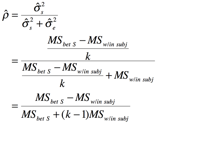
And, for the case with k = 2 observations per couple, the k - 1 term drops out.
An important thing to notice here is that MSw/in subj will not be affected by which score you put in column 1, and which goes in column 2. The variance of 45 and 49 is exactly the same as the variance of 49 and 45. Thus the order of assignment is irrelevant to the statistical result, which is exactly what we want.
The derivation above, which is essentially the same as that of Shrout and Fleiss (1979), leads to the following formula for the intraclass correlation coefficient.
Notice that I keep hopping back and forth between "couple," which is the term we would use from our example, and "subject," which is the way the analysis of variance would refer to this effect.
I have created a set of data for 50 couples that resembles the example above. These data are available at PartnerCorr.dat or at PartnerCorr.sav. I will set up the analysis in SPSS as a repeated measures analysis of variance, though I will completely ignore the effect due to Partners. The two most relevant dialogue boxes are shown below.(The breakdown to Partners is only needed so that I can add the components back together to get a within-subjects term.
I will set this up in a more traditional summary table. However, in a traditional table the term that we have labeled "Couple" is normally called "Subjects," and that is the notation that I will use here. Notice that the only reason for having a Partner and Error term is to allow them be to add them together to obtain the Within Subjects term. Also note that what SPSS calls the Error term in the Between- Subjects part of the table is what we would normally call the Between Subjects term. With these changes we obtain the following table.
Source df SS MS F Between Subj 49 14113.810 288.037 Within Subj 50 1567.500 31.350 Partner 1 13.690 13.690 Error 49 1553.810 31.710
From the formula given above we have
Thus our estimate of the correlation of sociability scores between partners in gay couples is .80. (These are fictitious data, and I don't know what the true correlation would be.)
If you are using SPSS to analyze your data, there is an easier way to calculate this coefficient. The advantage of this approach is that it also produces a confidence interval on our estimate.
The procedure that we want is the Reliability procedure, which is an old procedure in SPSS. In Version 21 that procedure can be found under Analyse/Scale/Reliability.
First chose that procedure from the menu. That will produce the following dialog box.
Notice that I have included the two variables (Part1 and Part2). You next need to click on the Statistics box, which will give you
Here I have selected the intraclass correlation coefficient, and then selected the One-Way Random model. (That is important--you don't want to take the default option.) Although in this image I have not selected the F test under "Anova table," I suggest that you do so. That is what I did on the more general page mentioned above.
The results are shown below.
Here you can see that the intraclass correlation agrees perfectly with the measure that we calculated (.804). The "Average Measure Intraclass Correlation" is not relevant to this particular problem. It represents our estimate of the reliability if we averaged the scores of the two partners, and used that as a variable. It can be obtained directly from the intraclass correlation coefficient by using the Spearman-Brown Prophecy formula (rSB = [(2*ricc)/(1+ricc)].
For those who would prefer to calculate the coefficient using R, the code is shown below. This is one of the simplest pieces of code for R that I have ever seen. The output follows that. In this particular case, the result that you want is given as ICC1. The other values are the same, but that is because of the nature of the problem. They will usually be different.
   data <- read.table (file.choose(), header = TRUE)
   coeff <- ICC(data)
   print(coeff)

   Intraclass correlation coefficients
                         type  ICC   F df1 df2       p lower bound upper bound
Single_raters_absolute   ICC1 0.80 9.2  49  50 4.1e-13        0.68        0.88
Single_random_raters     ICC2 0.80 9.1  49  49 7.9e-13        0.68        0.88
Single_fixed_raters      ICC3 0.80 9.1  49  49 7.9e-13        0.68        0.88
Average_raters_absolute ICC1k 0.89 9.2  49  50 4.1e-13        0.81        0.94
Average_random_raters   ICC2k 0.89 9.1  49  49 7.9e-13        0.81        0.94
Average_fixed_raters    ICC3k 0.89 9.1  49  49 7.9e-13        0.81        0.94

 Number of subjects = 50     Number of Judges =  2
An alternative function in R is the irr library. In our case we would ask for the oneway model. The commands and output are simply
 library(irr)
 icc(data)
 Single Score Intraclass Correlation

   Model: oneway
   Type : consistency

   Subjects = 50
     Raters = 2
     ICC(1) = 0.804

 F-Test, H0: r0 = 0 ; H1: r0 > 0
   F(49,50) = 9.19 , p = 4.1e-13

 95%-Confidence Interval for ICC Population Values:
  0.679 < ICC < 0.883
For a more complete discussion of alternative forms of ICC, please see icc-overall.html.
Griffin, D., & Gonzalez, R. (1995). Correlational analysis of dyad-level data in the exchangeable case. Psychological Bulletin, 118, 430-439
Field, A. P. (2005) Intraclass correlation. In Everitt, B. S. & Howell, D.C. Enclyopedia of Statistics in Behavioral Sciences . Chichester, England; Wiley.
McGraw, K. O. & Wong, S. P. (1996) . Forming inferences about some intraclass correlation coefficients. Psychological Methods, 1, 30 - 46.
On http://www.uvm.edu/~dhowell/StatPages/More_Stuff/icc/icc.html you admit that you don't know why the intraclass correlation formula is not a squared formula. How does the following explanation sound to you?
First consider the usual linear correlation. Although this is rarely made clear to statistics students-the correlation is not only the slope of the regression line when the two measurements are scaled to have equal spread, but it also measures how tightly the cloud of points is packed around the line of slope 1. When both measurements are scaled to have a standard deviation of 1, the average of the squared perpendicular distance to the line for the points is equal to 1 minus the absolute value of the correlation (Weldon 2000). This means that the larger the correlation, the tighter the packing.
Now consider an intraclass correlation for groups of size 2. When the whole set of measurements is scaled to have a standard deviation of 1, the average of the squared perpendicular distance to the slope of 1 line for the points is equal to 1 minus the intraclass correlation-- the exact parallel of the situation for the usual linear correlation. This means that the larger the intraclass correlation, the tighter the packing of the within-groups points to the line, and the higher the proportion of the variance of the whole data set is along the line (among the group means).
The source of the confusion may be that the usual linear correlation squared is the proportion of variance not "accounted for" by the regression line, so we tend to think of correlations in terms of square roots of something involving variances. But the correlation is just the covariance when the two variables are scaled to have SD =1, not the square root of the covariance. The plea of ignorance might be why is the proportion of variance not "accounted for" by the regression line equal to the linear correlation squared, not to the linear correlation?
Last modified 06/26/2015