

An important statistic that is integral to a significant portion of our research deals with reliability. If we are going to subjectively rate our subjects on any dimension, we want to know what degree of confidence we can assign to those ratings. And ratings can differ for a variety of reasons, some of which are not particularly import to us for the problem we are studying, and some of them are quite important. If you and I each rated 15 people on intellectual responsiveness, it is conceivable that you will rate each of those people about 5 points higher than I will. We agree on the relative weights--who is the best, who is the second best, who is the worst, and so on, but I just have a mental scale that is lower than yours. That might not be a problem in some research and might be a problem in other work. Or perhaps neither of us has a good idea of what "intellectual responsiveness" is, and our relative rankings of people may be entirely out of line with each other. That is a serious problem for almost any research study.
But there are other ways that our ratings can be viewed. In many cases we consider the subjects whose behavior is being rated as a random sample from some large pool of subjects. On the other hand, if we are working to train our raters so that they can participate in an upcoming study with these same subject, then these are the only subjects we care about and subjects will be considered as a fixed variable. Similarly, raters may be considered as either a random of a fixed variable. Each of these alternatives will lead to a different way of calculating our reliability coefficient, which will be an intraclass correlation.
There are a number of different intraclass correlations, and the classic reference is Shrout and Fleiss (1979). The reference to Griffin and Gonzales (1995), given below, is another excellent source.
It is simplest to think of a correlation involving two columns of ratings, one by rater#1 and the other by rater#2. (We are not limited to two columns of ratings, but I will assume that for the time being.) Moreover, I need not be restricted to columns of the actual raters doing the rating. I could have a column of scores of physical attrctiveness and another column of scores of popularity, but I won't go off in that direction here. See the discussion of ratings of sociability of same-sex partners.
As I said at the beginning, there are several kinds of intraclass correlations. They relate to different ways of conceptualizing the variables that are often referred to generically as "subjects" and "judges." Either of these variables may be a random variable (their levels were chosen at random from a population of possible levels) or a fixed variable, the different levels of which were specifically selected for this design, and the same levels would be selected again in a replication. In addition, we could use individual ratings, or we could take the mean of a set of ratings by different raters. Doing so will alter the intraclass correlation coefficient by providing a more reliable measure.
I have chosen to use the example of Shrout and Fleiss because the wonderful example that I dreamed up gave virtually the same answer for each model, and that will never do. In their example there are k = 4 judges and n = six subjects. The data are shown below. I did not put them in a separate data file because there are so few numbers that you can easily enter them by hand.
Subj Judge1 Judge2 Judge3 Judge4 1
2
3
4
5
6
9
6
8
7
10
62
1
4
1
5
2
5
3
6
2
6
48
2
8
6
9
7
For the design which I am discussing, with n = 6 subjects and k = 6 judges rating each subject, we have a matrix or data frame with n rows and k columns. I will label the people doing the rating as "judges," simply because that is in line with common descriptions. The value on the rows I will call "subjects."
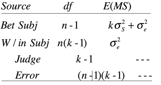
Shrout & Fleiss (1979) start with this simple example where n = 6 subjects are each rated by a different set of k = 4 judges. For example you might be looking at a sample of college applications, where each applicant is rated by four teachers (judges). It is important to note that for out first example different students would be rated by a different set of judges because they went to different schools, and judges would be considered to be a random variable from a huge population of potential teachers. You could think of this as an analysis of variance problem with 4 "groups" (teachers ) and 6 "subjects" (applicants). Applicants are considered a random variable sampled from a population of potential applicants. We cannot calculate a judge effect because each of the 4*6 = 24 different judges have only one score. Such a sum of squares would be exactly the same as SStotal. The following table of expected mean squares is adapted from one by Shrout and Fliess. (In the good old days when I was a graduate student we spent a lot more time worrying about expected mean squares than we do now. The advantage of thinking in those terms is that it allows you to derive formulae to fit particular relationhips, which is why I am taking that route here.
For the case that we are examining here, we will define the intraclass correlation as the ratio of the variance attributable to subjects divided by the total of subject and error variances. If the ratings by the four raters are in perfect agreement, there will be no within-subject variation, and hence no error variance, and that ratio will simply involve a variance term for subjects divided by a variance term for subjects plus a variance term for error, the latter being exactly 0. So the ratio will turn out to be 1.0. On the other hand, if there is little or no agreement between raters, the subject term may be quite small, our error term will be large, and the ratio will be somewhere near 0.0. That ratio is our intraclass correlation coefficient.
Our intraclass correlation coefficient for the study design that I have described will then be computed as
In terms of the analysis of variance, we have the total variation, (SStotal), which is the variation of all 24 ratings, without regard to whom they belong. We also have a Between Subject sum of squares, (SSsubjects), due to the fact that different students (the rows) have different ratings. Because we can't calculate a mean square due to judges, we have a one-way design in that we have only one meaningful dimension, i.e., Subjects, and that is a random variable.
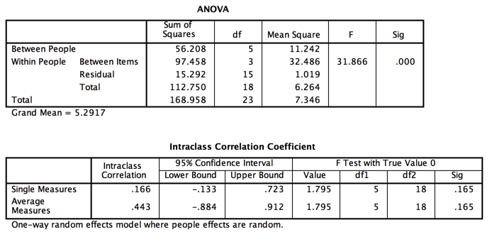
Using the formula given above, we can compute our estimate of the intraclass correlation using the analysis of variance table (from the analysis of variance given by SPSS) which appears below.
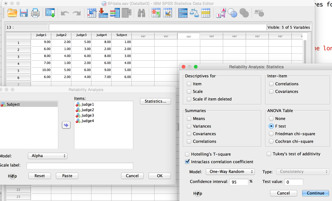
The screens and result from SPSS are shown below, followed by a similar result from R. I am only giving the illustration of the drop down menus from SPSS once, because I think that you can figure out the rest. I am using SPSS here because it gives you both the analysis of variance summary table and the computed result.
If we use the Scale/Reliability analysis from SPSS we obtain the following--notice how cleverly I got that all in one image!
In this analysis I have asked for a one-way random model because subjects are a random variable, and there is no meaningful sum of squares for judges, who only rate one student once. Notice also that I requested an analysis of variance summary table. That output is shown below.
Using the summary table given just above, we calculate the icc by hand from the equation that Shrout and Fliess give. That calculation is shown above the first SPSS screen.
The following is the result from R using the "icc" function in the "psych" library.
library(psych)
sfdata <- matrix(c(9,    2,   5,    8,
               6,    1,   3,    2,
               8,    4,   6,    8,
               7,    1,   2,    6,
               10,   5,   6,    9,
               6,   2,   4,    7),
		ncol=4,byrow=TRUE)
icc(ratings = sfdata, model="oneway",type = "consistency", unit = "single")

- - - - - - - - - - - - - - - - - - - - - - - - -
icc(ratings = sfdata, model = "oneway", type = "consistency", unit = "single")
 Single Score Intraclass Correlation

   Model: oneway
   Type : consistency

   Subjects = 6
     Raters = 4
     ICC(1) = 0.166

 F-Test, H0: r0 = 0 ; H1: r0 > 0
    F(5,18) = 1.79 , p = 0.165

 95%-Confidence Interval for ICC Population Values:
  -0.133 < ICC < 0.723
Alternatively,we can use the ICC function in the "irr" library to compute multiple types of intraclass correlation at once. This is shown below.
library(irr)
sfdata <- matrix(c(9,    2,   5,    8,
               6,    1,   3,    2,
               8,    4,   6,    8,
               7,    1,   2,    6,
               10,   5,   6,    9,
               6,   2,   4,    7),ncol=4,byrow=TRUE)
>  ICC(sfdata)

- - - - - - - - - - - - - - - - - - - - - - - - - - - - - - -
Call: ICC(x = sfdata)

Intraclass correlation coefficients
                         type  ICC    F df1 df2       p lower bound upper bound
Single_raters_absolute   ICC1 0.17  1.8   5  18 0.16477      -0.133        0.72
Single_random_raters     ICC2 0.29 11.0   5  15 0.00013       0.019        0.76
Single_fixed_raters      ICC3 0.71 11.0   5  15 0.00013       0.342        0.95
Average_raters_absolute ICC1k 0.44  1.8   5  18 0.16477      -0.884        0.91
Average_random_raters   ICC2k 0.62 11.0   5  15 0.00013       0.071        0.93
Average_fixed_raters    ICC3k 0.91 11.0   5  15 0.00013       0.676        0.99

 Number of subjects = 6     Number of Judges =  4
Suppose that we modify the design in the above example by making the same four judges rate all of the subjects. Further assume that those judges are somehow chosen at random--i.e. judges are a random variable. This is probably pushing things a bit in our specific example, but there are many cases where we would have such a design.
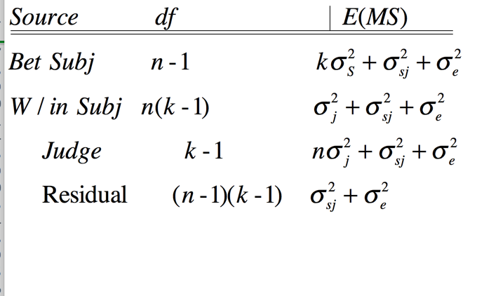
The expected mean squares for the design specified here is different from the ones that we had before, due to the fact that a meaningful term for judges can be derived because each judge rates multiple subjects. A modification of a table from Shroutt and Fleiss (1979) follows.
We will use the same basic analysis of variance, but under this design, with this set of expected mean squares, we have the following computation for the intraclass correlation coefficient.
For the final design that I want to talk about, let us consider the case where judges are a fixed variable. This could often arise if you are trying to train a set of graduate students to do ratings of subjects. These are not randomly chosen judges, but a specific set that are going to be working on this project. You just want them to be rating the same way. Again, the subjects will be a random variable, so we have a mixed model--one random variable and one fixed variable.
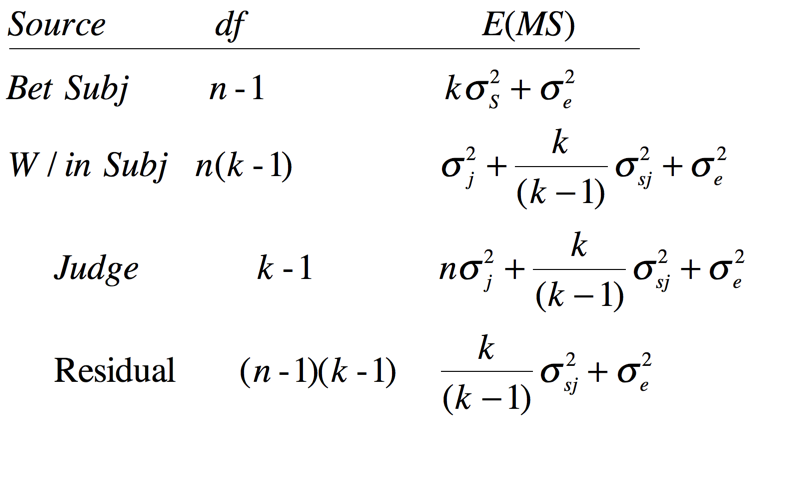
In this case the expected mean squares are a bit messier, not impossible. Shrout and Fleiss (1979) give them as:
This leaves us with the following definition of the intraclass correlation coefficient.
You will notice that in the printout I just showed you from the "irr" library and the "ICC" function, there were three extra lines, labelled "Average....". They are also intraclass correlations, but they are based on data where each rating is calculated as a mean of k ratings. In other words we will use k judges, but our final score for each subject will be the mean of those judges' ratings. I will not give those formulae here, but by looking at the output immediately above, you can see that those icc values will be higher than the values given by the corresponding first three solutions. That does not strike me as surprising, as the denominators in each case are smaller than in original solutions. The basic coefficients are derived from the formulae above, but substituting a value of 1 for k. This will cause some of the terms to drop out. If you need those solutions, see the reference by Shrout and Fliess.
Griffin, D., & Gonzalez, R. (1995). Correlational analysis of dyad-level data in the exchangeable case. Psychological Bulletin, 118, 430-439
Field, A. P. (2005) Intraclass correlation. In Everitt, B. S. & Howell, D.C. Enclyopedia of Statistics in Behavioral Sciences . Chichester, England; Wiley.
McGraw, K. O. & Wong, S. P. (1996) . Forming inferences about some intraclass correlation coefficients. Psychological Methods, 1, 30 - 46.
On http://www.uvm.edu/~dhowell/StatPages/More_Stuff/icc/icc.html you admit that you don't know why the intraclass correlation formula is not a squared formula. How does the following explanation sound to you?
First consider the usual linear correlation. Although this is rarely made clear to statistics students-the correlation is not only the slope of the regression line when the two measurements are scaled to have equal spread, but it also measures how tightly the cloud of points is packed around the line of slope 1. When both measurements are scaled to have a standard deviation of 1, the average of the squared perpendicular distance to the line for the points is equal to 1 minus the absolute value of the correlation (Weldon 2000). This means that the larger the correlation, the tighter the packing.
Now consider an intraclass correlation for groups of size 2. When the whole set of measurements is scaled to have a standard deviation of 1, the average of the squared perpendicular distance to the slope of 1 line for the points is equal to 1 minus the intraclass correlation-- the exact parallel of the situation for the usual linear correlation. This means that the larger the intraclass correlation, the tighter the packing of the within-groups points to the line, and the higher the proportion of the variance of the whole data set is along the line (among the group means).
The source of the confusion may be that the usual linear correlation squared is the proportion of variance not "accounted for" by the regression line, so we tend to think of correlations in terms of square roots of something involving variances. But the correlation is just the covariance when the two variables are scaled to have SD =1, not the square root of the covariance. The plea of ignorance might be why is the proportion of variance not "accounted for" by the regression line equal to the linear correlation squared, not to the linear correlation?
Last modified
dch