
Overview of Mixed Models
David C. Howell

Some time ago I wrote two web pages on using mixed-models for repeated measures designs. Those pages can be found at
Mixed-Models-for-Repeated-Measures1.html
and
Mixed-Models-for-Repeated-Measures2.html. This page, or perhaps set of pages, is designed for a different purpose. I am trying to sort out mixed models so that the average reader can understand their purpose and their relationship to one another. This involves focusing on fixed and random models and on repeated measures, and trying to explain why they go together.
Just about every source you read on these models takes a somewhat different approach, and it is not always clear how they relate to each other and why they look at the models so differently. One way to uderstand what is going on, if only vaguely, is to understand that the traditional analyses of variance assumes independent observations, or, with repeated measures, compound symmetry. This suggests that observations within the same group should be uncorrelated, or correlated in an unrealistic way. That's fine if you have just a bunch of random subjects, but it creates problems when you have repeated measures or you have independent variables nested within other independent variables. I want to try to sort this out. In addition, standard analyses of variance become controversial when you have unbalanced designs, meaning unequal cell sizes.
There are many books written on this topic, but each seems to take a slightly different approach and you sometimes end up wondering what they have to do with the problem you are trying to address. On top of that, different books and articles use different software, and a discussion written for SAS looks, on the surface, quite different from one written with respect to R. I can't cover everything, so I will first focus on SPSS, which uses a graphical user interface, and R, which is becoming more and more common, but does not have a GUI that will handle much of what I will cover here. Later on I will move to SAS
Perhaps my favorite source for mixed models is Maxwell and Delany (2004) Designing Experiments and Analyzing data (Chapter 15). They have done a particularly good job of working through the meaning of such designs, and are quite interpretable. For those interested in working through this material using R, there is a really excellent, and fairly brief, discussion of these models in a tutorial by Bodo Winter. It is entitled A very basic, and excellent, tutorial for performing linear mixed effects analyses, and can be downloaded at http://www.bodowinter.com/tutorials.html. You want the second tutorial, but it wouldn't hurt to read the first one as well.
Fixed and Random Variables
But what do we mean by mixed models? And how do repeated measures enter the discussion? And then what about nested effects? All of these topics have a role in this discussion, and sorting them out in a meaningful way has proved to be difficult. Part of my difficulty is that I wanted to come at this topic from the direction of an anlysis of variance, with which you probably have some reasonably familiarity. There are situations under which the analysis of variance and maximum likelihood, the major tool for mixed models, produce the same result. It is therefore tempting to start with Anova and then move on. But I have been forced to give up on that approach simply because it leads me down too many alleys at the same time. Instead, I am going to go at the issues head on.
You might think that the distinction between fixed and random variables is something that statisticians worked out years ago. But actually there is still a good bit of discussion about them. There are two issues here. First, what is the difference between fixed and random variables, and second, how do we estimate their effects and why are they different.
If you want to run a study to compare the effects of four different drugs on the treatment of depression, you will want to treat Drugs as a fixed effect. You have deliberately selected those drugs and not others, and your interest is just in their effects. Put a different way, you want to focus on the differences between groups. You are not planning to generalize to other drugs. In the field of experimental psychology this is the way that we ran most of our experiments, and fixed effects were the basic building blocks.
The designs that we often use for a standard analysis of variance include one random variable, normally "subjects," but this is often about it. A random variable can be thought of as a variable whose levels were chosen at random. Alternatively, some would argue that a random variable is one for which you want to make a global statement about the population of levels. When we apply an experiment to many different classrooms, we really aren't particularly interested in saying that Miss Smith's class is better than Mr. Jones' class. We want to make a general statement about the variability among classrooms, as opposed to statements like Drug A is a better treatment for depression than Drug B, which is what we want for fixed variables.
But this last statement brings me to another distinction that will color the output we receive and, in some ways, make the printout from most software analyses look as if the distinction from the analysis of variance is even greater than it is. In the analysis of variance approach, even when our model has a random experimental variable, we expect to see a summary table that emphasizes F tests on each of the effects. In other words, we expect to see output that says there are significant differences due to A, perhaps no differences due to B, and perhaps a significant interaction. Then we flesh out what those mean, perhaps with multiple comparison tests, effect sizes, and so on, and stop. But in a mixed model you will see that we pull apart fixed factors from random factors, present a significance test on the fixed factors, if we can figure out how to do that, and then compute and focus on the variance of the random factors. So our resulting output has two quite different parts. And this really does make sense. I want to know if Drug A is a better treatment than Drug B, but I don't particularly want to know that Mary is better than John--although I might want to make a statement about how variable subjects are in general. So expect to see output that is in many ways different from what you are used to.
There is at least one more feature of mixed-models that makes things look quite different. In Howell (1913 - Chapter 13) I show that with a balanced design, which generally means equal cell sizes, we can work out expected mean squares, figure out how to compute F values for fixed effects, and go our merry way. But in the general case where we often don't have nice balanced designs, our statistical test for that fixed effect will often boil down to a chi-square test comparing a full and reduced model, where the reduced model omits the factor in question. That makes it look as if we have gone a long way in a different direction. We really haven't, but it certainly looks that way.
Independence of Observations
You probably know that for a standard analysis of variance we assume that observations are independent. Or, when it comes to repeated measures, we assume sphericity or compound symmetry. But for repeated measures designs in particular, those are frequently not reasonable assumptions. In the standard analysis of variance we dropped back to corrections by Huynh and Feldt (1970) or Greenhouse and Geisser (1958). But those are only approximations. With mixed models we no longer have to make a compound symmetry assumption, so we can avoid approximations. You will see how to do that later. But I need to say a bit more about this here because it is a central aspect of dealing with mixed models.
It is easier to see what the problem is with assuming independence if we look at a repeated measure. Suppose that we follow a group of patients by testing them every month for six months. If we had compound symmetry, a standard repeated measures assumption, then the correlation between patients' data at Time 1 and Time 2 would be the same as the (expected) correlation between the data on Time 1 and Time 5. But is that reasonable? Don't you think that your subjects' Time 1 and Time 2 scores will be more highly correlated that their Time 1 and Time 5 scores. In other words data collected closer in time will be more similar than data collected further apart in time? But if that is the case, we won't have compound symmetry. As I said, we can, on occasion, fall back on correction factors such as those of Greenhouse and Geisser or Huhyn and Feldt, but those are not always satisfactory either. But with our new analysis of choice, maximum likelihood, we can find other ways around this problem that give a better solution.
SPSS and R
For at least the first part of this page I am going to base my analyses on the SPSS package and on R. SPSS has the advantage (???) of offering a graphical user interface to help you set up your analysis. It is also widely available, expecially on university campuses. At the moment, R's lme4() package does not allow you to specify alternative correlational structures, although you can specify that the slopes for each individual over time are assessed separately.
But, while a graphical user interface is generally easier to use, I don't find it all that easy with the mixed models analysis. But I found a very good discussion of using that interface in a chapter by Howard Seltman at CMU, which is available on line at http://www.stat.cmu.edu/~hseltman/309/Book/chapter15.pdf. I think that he has done a very good job of explaining what you need to do. However in the SPSS code you see below, I have given you the syntax. You can simply paste that in to SPSS and run it from there. (Of course you need to do something about identifying the data set, but you can use the GUI to do that.) By the way, I strongly recommend that you go to Howard Seltman's home page at http://www.stat.cmu.edu/~hseltman/ and click on the link to "Statistics/Math." He has a wealth of amazing links to important articles and material on the web. In addition, he has a very complete FREE statistics text on the web at http://www.stat.cmu.edu/~hseltman/309/Book/Book.pdf. Check it out, although I hope that you think my book is better.
Example Data
My motivation for this document came from a question asked by Rikard Wicksell at Karolinska University in Sweden. He had a randomized clinical trial with two treatment groups and measurements at pre, post, 3 months, and 6 months. His problem is that some of his data were missing. He considered a wide range of possible solutions, including "last trial carried forward," mean substitution, and listwise deletion. In some ways listwise deletion appealed most, but it would mean the loss of too much data. One of the nice things about mixed models is that we can use all of the data we have. If a score is missing, it is just missing. It has no effect on other scores from that same patient.
Another advantage of mixed models is that we don't have to be consistent about time. For example, and it does not apply in this particular example, if one subject had a follow-up test at 4 months while another had their follow-up test at 5 months, we simply enter 4 (or 5) as the time of follow-up. We don't have to worry that they couldn't be tested at the same intervals.
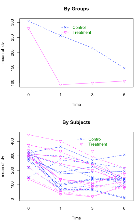
I have created data to have a number of important characteristics. (These are my own fabricated data, and should not be taken as the data that Wicksell found.) There are two groups - a Control group and a Treatment group, measured at 4 times. These times are labeled as 0 (pretest), 1 (one month posttest), 3 (three months follow-up), and 6 (six months follow-up). Both Group and Time are fixed variables. I created the treatment group to show a sharp drop at post-test and then sustain that drop (with slight regression) at 3 and 6 months. The Control group declines slowly over the 4 intervals but does not reach the low level of the Treatment group. There are noticeable individual differences in the Control group, and some subjects show a steeper slope than others. In the Treatment group there are individual differences in level but the slopes are not all that much different from one another. You might think of this as a study of depression, where the dependent variable is a depression score (e.g. Beck Depression Inventory) and the treatment is drug versus no drug. If the drug worked about as well for all subjects the slopes would be comparable and negative across time. For the control group we would expect some subjects to get better on their own and some to stay depressed, which would lead to differences in slope for that group. These facts are important because with random variables the individual differences will show up as variances in subjects' intercepts, and any slope differences will show up as a significant variance in the slopes. The only random variable in this particular example is "Subjects."
The data used below are available (with no missing values) at WicksellLongComplete.dat. I need to say something important about the structure of the data. If you were planning on running a standard analysis of variance, you would most likely put each subject's data on a single line. You would probably have Subject Number, Group, Time1, Time2, Time3, and Time4 all sitting side by side. That is generally referred to as the "wide format." But for what we will be doing, we will use what is called the "long format." There will be a separate line for each dependent variable... In other words, we will have a column for Subject Number, one for Time (represented as 0, 1, 3, or 6), one for Group, and one for the dependent variable. Then we will go to the next line, enter the same Subject Number, the same Group, a "1" for Time2, and then the Time2 measure. This data file is shown below, although to save space here I have typed it as three separate columns rather than display it all in one very long table with one line of variable names and 96 lines of data.
| Subj Time Group dv
1 0 1.00 296.00
1 1 1.00 175.00
1 3 1.00 187.00
1 6 1.00 192.00
2 0 1.00 376.00
2 1 1.00 329.00
2 3 1.00 236.00
2 6 1.00 76.00
3 0 1.00 309.00
3 1 1.00 238.00
3 3 1.00 150.00
3 6 1.00 123.00
4 0 1.00 222.00
4 1 1.00 60.00
4 3 1.00 82.00
4 6 1.00 85.00
5 0 1.00 150.00
5 1 1.00 271.00
5 3 1.00 250.00
5 6 1.00 216.00
6 0 1.00 316.00
6 1 1.00 291.00
6 3 1.00 238.00
6 6 1.00 144.00
7 0 1.00 321.00
7 1 1.00 364.00
7 3 1.00 270.00
7 6 1.00 308.00
8 0 1.00 447.00
8 1 1.00 402.00
8 3 1.00 294.00
8 6 1.00 216.00
|
9 0 1.00 220.00
9 1 1.00 70.00
9 3 1.00 95.00
9 6 1.00 87.00
10 0 1.00 375.00
10 1 1.00 335.00
10 3 1.00 334.00
10 6 1.00 79.00
11 0 1.00 310.00
11 1 1.00 300.00
11 3 1.00 253.00
11 6 1.00 140.00
12 0 1.00 310.00
12 1 1.00 245.00
12 3 1.00 200.00
12 6 1.00 120.00
13 0 2.00 282.00
13 1 2.00 186.00
13 3 2.00 225.00
13 6 2.00 134.00
14 0 2.00 317.00
14 1 2.00 31.00
14 3 2.00 85.00
14 6 2.00 120.00
15 0 2.00 362.00
15 1 2.00 104.00
15 3 2.00 144.00
15 6 2.00 114.00
16 0 2.00 338.00
16 1 2.00 132.00
16 3 2.00 91.00
16 6 2.00 77.00
|
17 0 2.00 263.00
17 1 2.00 94.00
17 3 2.00 141.00
17 6 2.00 142.00
18 0 2.00 138.00
18 1 2.00 38.00
18 3 2.00 16.00
18 6 2.00 95.00
19 0 2.00 329.00
19 1 2.00 62.00
19 3 2.00 62.00
19 6 2.00 6.00
20 0 2.00 292.00
20 1 2.00 139.00
20 3 2.00 104.00
20 6 2.00 184.00
21 0 2.00 275.00
21 1 2.00 94.00
21 3 2.00 135.00
21 6 2.00 137.00
22 0 2.00 150.00
22 1 2.00 48.00
22 3 2.00 20.00
22 6 2.00 85.00
23 0 2.00 319.00
23 1 2.00 68.00
23 3 2.00 67.00
23 6 2.00 12.00
24 0 2.00 300.00
24 1 2.00 138.00
24 3 2.00 114.00
24 6 2.00 174.00
|
Interaction Plot, First by Groups, and then by Subjects within Groups
To give a starting point for the analyses that follow, I have included the SPSS and R code that would run the appropriate analysis. With balanced data this analysis is just fine, which is why I use it as a starting point, but you are going to see that we will vary the code as we go along. Notice several things in the code that follows. In SPSS I have to specify that the independent variables of Time and Group are nominal variables. In R they need to be specified as factors. I first need to convert the independent variables to factors. Otherwise the analysis would treat Time as a continous measure with 1 df instead of 4 levels. But I am also going to need time as a continuous measure in later analyses, so I also create the continuous Time.cont variable before modifying Time to a factor. In SPSS be sure that you specify that this is a scaled variable.
DATASET ACTIVATE DataSet4.
COMPUTE Time.cont=Time.
EXECUTE.

MIXED dv BY Group Time
  /CRITERIA=CIN(95) MXITER(100) MXSTEP(10) SCORING(1) SINGULAR(0.000000000001) HCONVERGE(0,
    ABSOLUTE) LCONVERGE(0, ABSOLUTE) PCONVERGE(0.000001, ABSOLUTE)
  /FIXED=Group Time Group*Time | SSTYPE(3)
  /METHOD=REML
  /REPEATED=Time | SUBJECT(Subject) COVTYPE(CS).
If I ran the same analysis Using R, I would use the following code and obtain the results shown below. You will see that the results look exactly like those of SPSS except for the -2 Restricted Log Likelihood. I do not know why they differ. They both call for REML, so they should be the same. Go Figure!
If you look at the output for fixef(model2), you will first obtain the intercept, which is the grand mean of dv, and then the group and cell effects, which are their deviations from the grand mean or, for example, mean(dv) - mean(Group1) - mean(Time1) + mean(Cell11). If you look at the random effects with ranef(model2), you will see the individual intercepts for each subject.
# Analysis of Wicksell Data with complete data
rm(list = ls())
server <-  "http://www.uvm.edu/~dhowell/StatPages/DataFiles/"
dataComplete <- read.table(paste0(server, "WicksellLongComplete.dat"), header = TRUE)
dataComplete <- within(dataComplete, {
   Time.cont <- Time     #A continuous (or at least ordered) variable
   Time = factor(Time)
   Group = factor(Group)
   Subject = factor(Subject)
})
options(contrasts = c("contr.sum","contr.poly"))
library(lme4)
library(car)
library(lmerTest)    # An approach to obtaining p values
model2 <- lmer(dv~Group + Time + Time:Group + (1|Subject), REML = TRUE, data = dataComplete)
summary(model2)
anova(model2)

### Interaction plot
with(dataComplete, {     ## Need this because interaction.plot will
#                        ## not take"data = dataComplete"
   par(mfrow = c(2,1))
   interaction.plot(Time, factor(Group), dv, type="b", pch = c(4,6),
                    legend = "F", col = c(4,6))
   legend(2, 300, c("Control",  "Treatment"), col = c(4,6),
          text.col = "green4", lty = c(2, 1, 3), pch = c(4, 6),
          merge = TRUE, bty = "n")
})

#### Output

> summary(model2)
Linear mixed model fit by REML t-tests use Satterthwaite approximations to degrees
of freedom [lmerMod]
Formula: dv ~ Group + Time + Time:Group + (1 | Subject)
   Data: dataComplete

REML criterion at convergence: 1011.9
Scaled residuals:
     Min       1Q   Median       3Q      Max
-2.79300 -0.38860  0.00641  0.55955  1.76696

Random effects:
 Groups   Name        Variance Std.Dev.
 Subject  (Intercept) 2539     50.39
 Residual             2761     52.54
Number of obs: 96, groups:  Subject, 24

Fixed effects:
             Estimate Std. Error      df t value Pr(>|t|)
(Intercept)   188.437     11.600  22.000  16.244 9.77e-14 ***
Group1         42.958     11.600  22.000   3.703 0.001240 **
Time1         103.938      9.288  65.990  11.190  < 2e-16 ***
Time2         -12.854      9.288  65.990  -1.384 0.171041
Time3         -30.396      9.288  65.990  -3.273 0.001698 **
Group1:Time1  -31.000      9.288  65.990  -3.338 0.001392 **
Group1:Time2   38.125      9.288  65.990   4.105 0.000114 ***
Group1:Time3   14.750      9.288  65.990   1.588 0.117055

Correlation of Fixed Effects:
            (Intr) Group1 Time1  Time2  Time3  Gr1:T1 Gr1:T2
Group1       0.000
Time1        0.000  0.000
Time2        0.000  0.000 -0.333
Time3        0.000  0.000 -0.333 -0.333
Group1:Tim1  0.000  0.000  0.000  0.000  0.000
Group1:Tim2  0.000  0.000  0.000  0.000  0.000 -0.333
Group1:Tim3  0.000  0.000  0.000  0.000  0.000 -0.333 -0.333
> anova(model2)
Analysis of Variance Table of type III  with  Satterthwaite
approximation for degrees of freedom
           Sum Sq Mean Sq NumDF  DenDF F.value    Pr(>F)
Group       37860   37860     1 22.000  13.714   0.00124 **
Time       373803  124601     3 65.971  45.135 5.551e-16 ***
Group:Time  74654   24885     3 65.971   9.014 4.384e-05 ***
NOTE: p values, df, and note about Sattertwaite caused by inclusiomn of permTest.
The information criteria given in the output of SPSS are measures of goodness of fit. We will return to these shortly. Notice that the summary table for the fixed effects is a standard analysis of variance table, complete with p values. I should also point out that SPSS allowed me to specify compound symmetry of the covariances, which results in the table of covariance parameters to give only one entry for the CS covariance element, because all of these covariances are assumed to be equal in the population.
Here we see that each of the effects in the overall analysis is significant. We don't care very much about the group effect because we expected both groups to start off equal at pre-test. What is important is the interaction, and it is significant at p = .0001. Clearly the drug treatment is having a differential effect on the two groups, which is what we wanted to see. The fact that the Control group seems to be dropping in the number of symptoms over time is to be expected and not exciting, although we could look at these simple effects if we wanted to. We would just run two analyses, one on each group. I would not suggest pooling the variances to calculate F, though that would be possible.
To go on one small amount, you can ask for different slopes by running the following model
# Now use the following model which allows for groups to have different slopes over time.
model3 <- lmer(dv ~ Group + Time + Time:Group  + (1 + Time.cont|Subject),data = dataComplete)
summary(model3)
anova(model3)
________________________________________________________
> anova(model3)
Analysis of Variance Table
           Df Sum Sq Mean Sq F value
Group       1  24214   24214  13.209
Time        3 222792   74264  40.513
Group:Time  3  73008   24336  13.276

> ranef(model3)
$Subject
    (Intercept)  Time.cont
1   -38.6682293   8.179511
2    61.4205448 -15.133844
3   -16.3448012  -2.048576
4  -126.2085949   9.507208
5   -55.5528555  16.985619
6    21.2135279  -2.845906
7    49.2291678   7.621402
8   123.0190152 -11.594094
9  -121.1508026   9.417902
10   81.9422138 -14.548133
11   24.8314030  -3.093139
...   	...	   ...
The printout for the random effects will show both different intercepts and different slopes for each subject. That is probably a more realistic analysis, because we would expect that different people would change in somewhat different ways over time. Notice that I had to use Time.cont to obtain the differences in slopes. That makes sense because if
time is just a categorical variable, how would you expect to calculate a slope with an arbitrary ordering of a variable?
But notice that the summary table for fixed effects is quite different from the one we get when we only ask for different intercepts.
There is at least one more final step. We have two models, one of which allows varying slopes across subjects while the other does not. We can compare these two models with another "anova" statement. This will produce a chi-square test on the difference between the two models. The result is given below, where we see that the model with varying slopes is a better fit to the data. (Of course, I created the data to have that effect.)
refitting model(s) with ML (instead of REML)
Models:
model2: dv ~ Group + Time + Time:Group + (1 | Subject)
model3: dv ~ Group + Time + Time:Group + (1 + Time.cont | Subject)
anova(model2, model3)
       Df    AIC    BIC  logLik deviance  Chisq Chi  Df   Pr(>Chisq)
model2 10 1081.8 1107.4 -530.87   1061.8
model3 12 1076.4 1107.2 -526.21   1052.4     9.3349   2   0.009396 **
Mixed Models and Missing Data
The final general point I will make about mixed models, actually about maximum likelihood, is that missing data present far fewer problems than they do with the analysis of variance. If a piece of data is missing, it is just missing and you go on. But in the analysis of variance with repeated measures, if a subject is missing a score on Trial 2, all of that person's data are left out of the analysis. Our analyses include only subjects with complete data. And that can do a serious job of distorting an analysis and it certainly eats into the degrees of freedom. So here is one very big plus for maximum likelihood.
In the section above I have computed a mixed model analysis. But with balanced data the result does, and should, come out just about the same. But now I want to go to a model with missing, and therefore unbalanced data. I use the same data set but deleted data pretty much at random. I took out nine data points from 7 cases. For a standard analysis of variance this would mean completely eliminating those nine cases, thus losing 9*4 = 36 observations. But with a maximum liklihood I can just lose the 9 missing data points. That's a big difference in itself. I have not reproduced the data, but they are available at http://www.uvm.edu/~dhowell/StatPages/Mixed-Models-Repeated/WicksellLongMiss.dat. Before going on, I show the same analyses that we just ran, but this time on the missing data.I will begin with SPSS printout calling for a Type III analysis assuming compound symmetry. This is shown below
SPSS
   Information Criteria
-2 Restricted Log Likelihood	        901.756
Akaike's Information Criterion (AIC)	905.756
Hurvich and Tsai's Criterion (AICC)	905.914
Bozdogan's Criterion (CAIC)	        912.495
Schwarz's Bayesian Criterion (BIC)	910.495
The information criteria are displayed in smaller-is-better form.
a Dependent Variable: dv.

Fixed Effects
Type III Tests of Fixed Effectsa
Source	Numerator df	Denominator df	    F	  Sig.
Intercept	1	    22.495	257.814	  .000
Time	        3	    58.546	 37.816	  .000
Group	        1	    22.495	 11.447	  .003
Time * Group	3	    58.546	  8.829	  .000
a Dependent Variable: dv.

Estimates of Covariance Parameters
Parameter		                        Estimate	      Std. Error
Repeated Measures	CS diagonal offset	2777.418969    	       518.006015
	                CS covariance	        2595.566062	      1020.806839
a Dependent Variable: dv.

AND NOW USING LMER FUNCTION FOR R.
#### With Missing Data
server <-  "http://www.uvm.edu/~dhowell/StatPages/DataFiles/"
data3 <- read.table("WicksellLongMissNA.dat", header = TRUE)  # WicksellLongMiss.dat
tail(data3)
data3$Group <- factor(data3$Group)
data3$Subject <- factor(data3$Subject)
data3$time.cont <- data3$Time
data3$Time <- factor(data3$Time)

### With random intercept
library(lme4)
model4 <- lmer(dv ~ Time*Group + (1|Subject), data = data3, contrasts = contr.sum)
summary(model4)
anova(model4, type = 3)

_______________________________________________________________

Analysis of Variance Table of type III  with  Satterthwaite
approximation for degrees of freedom
           Sum Sq Mean Sq NumDF  DenDF F.value    Pr(>F)
Time       315092  105031     3 58.556  37.816 1.008e-13 ***
Group       31792   31792     1 22.495  11.447  0.002617 **
Time:Group  73570   24523     3 58.556   8.829 6.424e-05 ***
---

_____________________________________________________________

### With random intercept and slope
model5 <- lmer(dv ~ Time*Group + (1+Time.cont|Subject), data = data3, contrasts = contr.sum)
summary(model5)
anova(model5, type = 3)
_____________________________________________________________

Analysis of Variance Table of type III  with  Satterthwaite
approximation for degrees of freedom
           Sum Sq Mean Sq NumDF  DenDF F.value    Pr(>F)
Time       219420   73140     3 35.132  38.725 3.093e-11 ***
Group       22138   22138     1 22.567  11.721  0.002367 **
Time:Group  65354   21785     3 35.132  11.534 2.056e-05 ***

REML criterion at convergence: 905

Scaled residuals:
    Min      1Q  Median      3Q     Max
-1.7011 -0.4973 -0.0079  0.5921  1.7712

Random effects:
 Groups   Name        Variance Std.Dev. Corr
 Subject  (Intercept) 5116.4   71.53
          Time.cont    125.9   11.22    -0.77
 Residual             1888.7   43.46
Number of obs: 87, groups:  Subject, 24

Fixed effects:
             Estimate Std. Error      df t value Pr(>|t|)
(Intercept)   189.897     11.883  22.570  15.981 8.57e-14 ***
Time1         102.478      9.809  44.580  10.447 1.45e-13 ***
Time2         -17.755      8.824  60.320  -2.012 0.048677 *
Time3         -30.149      8.401  42.810  -3.589 0.000849 ***
Group1         40.682     11.883  22.570   3.424 0.002367 **
Time1:Group1  -28.724      9.809  44.580  -2.928 0.005352 **
Time2:Group1   36.959      8.824  60.320   4.188 9.29e-05 ***
Time3:Group1   16.491      8.401  42.810   1.963 0.056177 .
---
Signif. codes:  0 ‘***’ 0.001 ‘**’ 0.01 ‘*’ 0.05 ‘.’ 0.1 ‘ ’ 1

Correlation of Fixed Effects:
            (Intr) Time1  Time2  Time3  Group1 Tm1:G1 Tm2:G1
Time1        0.234
Time2        0.151  0.037
Time3       -0.060 -0.323 -0.342
Group1      -0.018  0.021  0.036 -0.002
Time1:Grop1  0.021 -0.026 -0.043  0.002  0.234
Time2:Grop1  0.036 -0.043  0.002 -0.016  0.151  0.037
Time3:Grop1 -0.002  0.002 -0.016 -0.051 -0.060 -0.323 -0.342
If you ran lmer without loading the lmerTest() library, you will note that the F value for the interaction is the same in the two analyses, but the main effects are slightly different. This is because R, by default, performs a Type I analysis of variance, whereas SPSS uses Type III by default. However, the output I show has been created after loading lmerTest() and requesting Tytpe III an analysis, and it now produces, by default, Type III SS and matches SPSS exactly. (I don't know that Bates would be happy to have lmerTest() redesign the standard R analysis for lmer(), but that happens once you have loaded lmerTest. You don't even have to think about it. If you don't like this effect, you can enter "detach(package:lmerTest)."
If you look at the code given above for R, I asked R to allow each subject to have a different intercept. The way I have set this up, that means that they will start off a different levels. But I had not asked it to allow them have different slopes--i.e. change differentially over trials. So that is where I went next.
When I want R to allow different slopes for each subject, I have to code the command differently. Writing
model4 <- lmer(dv ~ Time*Group + (1|Subject), data = data3, contrasts = contr.sum)
says that I want a different intercept for each subject. That is what the "1" stands for. If I want a different slope, I need to write something like
lmer(dv ~ Group*Time + (1 + Time|Subject), data = data3 )
but that won't work if you just use "Time" to indicate random slopes, because in my code Time is a factor. Here is where that Time.cont comes in. It is a numeric variable, so you can have a slope for Time.cont. By default, you will also get different intercepts, whether or not you keep the "1."
Notice that allowing the slopes to vary over subjects produces a somewhat different result. However it is not greatly different. Notice that "summary(model5) shows us the variance of subjects and the variance of the slopes. This is what we would expect.
Other Covariance Structures
To this point all of our analyses have been based on an assumption of compound symmetry. (The assumption is really about sphericity, but the two are close and Proc Mixed refers to the solution as type = cs.) But if you look at the correlation matrix given earlier it is quite clear that correlations further apart in time are distinctly lower than correlations close in time, which sounds like a reasonable result. Also if you looked at Mauchly's test of sphericity (not shown) it is significant with p = .012. While this is not a great test, it should give us pause. We really ought to do something about sphericity.
In what follows, I am switching to SAS because it offers greater flexibility. (Immediately below this paragraph is the comparable syntax for SPSS using WicksellLongMiss.dat. You will need to change the covariance structure as SAS changes, but otherwise the outputs agree remarkably well.) The first thing that we could do about sphericity is to specify that the model will make no assumptions whatsoever about the form of the covariance matrix. To do this I will ask for an unstructured matrix. This is accomplished by including type = un in the repeated statement. This will force SAS to estimate all of the variances and covariances and use them in its solution. The problem with this is that there are 10 things to be estimated and therefore we will lose degrees of freedom for our tests. But I will go ahead anyway. For this analysis I will continue to use the data set with missing data, though I could have used the complete data had I wished. I will include a request that SAS use procedures due to Hotelling-Lawley-McKeon (hlm) and Hotelling-Lawley-Pillai-Samson (hlps) which do a better job of estimating the degrees of freedom for our denominators. This is recommended for an unstructured model. The results are shown below.
Comparable Syntax for SPSS

MIXED dv BY Group Time
  /CRITERIA=CIN(95) MXITER(100) MXSTEP(10) SCORING(1) SINGULAR(0.000000000001) HCONVERGE(0,
    ABSOLUTE) LCONVERGE(0, ABSOLUTE) PCONVERGE(0.000001, ABSOLUTE)
  /FIXED=Group Time Group*Time | SSTYPE(3)
  /METHOD=REML
  /REPEATED=Time | SUBJECT(Subject) COVTYPE(UN).
Results From SAS Using Unstructured Matrix
Proc Mixed data = lib.WicksellLongMiss;
   class group time subject;
   model dv = group time group*time ;
   repeated time /subject = subject type = un hlm hlps  rcorr;
run;


Estimated R Correlation Matrix for subject 1
 Row        Col1        Col2        Col3        Col4
   1      1.0000      0.5858      0.5424    -0.02740
   2      0.5858      1.0000      0.8581      0.3896
   3      0.5424      0.8581      1.0000      0.3971
   4    -0.02740      0.3896      0.3971      1.0000

Covariance Parameter Estimates

Cov Parm    Subject    Estimate
UN(1,1)     subject     5548.42
UN(2,1)     subject     3686.76
UN(2,2)     subject     7139.94
UN(3,1)     subject     2877.46
UN(3,2)     subject     5163.81
UN(3,3)     subject     5072.14
UN(4,1)     subject     -129.84
UN(4,2)     subject     2094.43
UN(4,3)     subject     1799.21
UN(4,4)     subject     4048.07

           Fit Statistics
-2 Res Log Likelihood           883.7
AIC (smaller is better)         903.7
AICC (smaller is better)        906.9
BIC (smaller is better)         915.5
-----------------------------------------------------------------------------------------

Same analysis but specifying an unstructured covariance matrix.

The Mixed Procedure
  Null Model Likelihood Ratio Test
    DF    Chi-Square      Pr > ChiSq
     9         40.92          <.0001


         Type 3 Tests of Fixed Effects

               Num     Den
Effect          DF      DF    F Value    Pr > F
group            1      22      17.95    0.0003
time             3      22      28.44    <.0001
group*time       3      22       6.80    0.0021

   Type 3 Hotelling-Lawley-McKeon Statistics

                Num     Den
Effect          DF      DF    F Value    Pr > F
time             3      20      25.85    <.0001
group*time       3      20       6.18    0.0038
----------------------------------------------------------------------------------------
Notice the matrix of correlations. From pretest to the 6 month follow-up the correlation with pretest scores has dropped from .46 to -.03, and this pattern is consistent. That certainly doesn't inspire confidence in compound symmetry.
The Fs have not changed very much from the previous model, but the degrees of freedom for within-subject terms have dropped from 57 to 22, which is a huge drop. That results from the fact that the model had to make additional estimates of covariances. Finally, the hlm and hlps statistics further reduce the degrees of freedom to 20, but the effects are still significant. This would make me feel pretty good about the study if the data had been real data.
But we have gone from one extreme to another. We estimated two covariance parameters when we used type = cs and 10 covariance parameters when we used type = un. (Put another way, with the unstructured solution we threw up our hands and said to the program "You figure it out! We don't know what's going on.' There is a middle ground (in fact there are many). We probably do know at least something about what those correlations should look like. Often we would expect correlations to decrease as the trials in question are further removed from each other. They might not decrease as fast as our data suggest, but they should probably decrease. An autoregressive model, which we will see next, assumes that correlations between any two times depend on both the correlation at the previous time and an error component. To put that differently, your score at time 3 depends on your score at time 2 and error. (This is a first order autoregression model. A second order model would have a score depend on the two previous times plus error.) In effect an AR(1) model assumes that if the correlation between Time 1 and Time 2 is .51, then the correlation between Time 1 and Time 3 has an expected value of .5122 = .26 and between Time 1 and Time 4 has an expected value of .5133 = .13. (For SPSS the comparable covariance structure is named "AR1".) Our data look reasonably close to that. (Remember that these are expected values of r, not the actual obtained correlations.) The solution using a first order autoregressive model follows.
Title 'Same analysis but specifying an autoregressive covariance matrix.';

Proc Mixed data = lib.WicksellLongMiss;
      class group subject time;
      model dv = group time group*time;
      repeated time /subject = subject type = AR(1) rcorr;
run;

Same analysis but specifying an autoregressive covariance matrix.

    Estimated R Correlation Matrix for subject 1

 Row        Col1        Col2        Col3        Col4
   1      1.0000      0.6182      0.3822      0.2363
   2      0.6182      1.0000      0.6182      0.3822
   3      0.3822      0.6182      1.0000      0.6182
   4      0.2363      0.3822      0.6182      1.0000


 Covariance Parameter Estimates

 Cov Parm     Subject    Estimate
AR(1)        subject      0.6182
Residual                 5350.25

           Fit Statistics
-2 Res Log Likelihood           895.1
AIC (smaller is better)         899.1
AICC (smaller is better)        899.2
BIC (smaller is better)         901.4

  Null Model Likelihood Ratio Test
    DF    Chi-Square      Pr > ChiSq
     1         29.55          <.0001


         Type 3 Tests of Fixed Effects

               Num     Den
Effect          DF      DF    F Value    Pr > F
group            1      22      17.32    0.0004
time             3      57      30.82    <.0001
group*time       3      57       7.72    <.0002
Notice the pattern of correlations. The .6182 as the correlation between adjacent trials is essentially an average of the correlations between adjacent trials in the unstructured case. The .3822 is just .618222 and .2363 = .618233. Notice that tests on within-subject effects are back up to 57 df, which is certainly nice, and our results are still significant. This is a far nicer solution than we had using Proc GLM.
Now we have three solutions, but which should we choose? One aid in choosing is to look at the "Fit Statistics' that are printed out with each solution. These statistics take into account both how well the model fits the data and how many estimates it took to get there. Put loosely, we would probably be happier with a pretty good fit based on few parameter estimates than with a slightly better fit based on many parameter estimates. If you look at the three models we have fit for the unbalanced design you will see that the AIC criterion for the type = cs model was 909.4, which dropped to 903.7 when we relaxed the assumption of compound symmetry. A smaller AIC value is better, so we should prefer the second model. Then when we aimed for a middle ground, by specifying the pattern or correlations but not making SAS estimate 10 separate correlations, AIC dropped again to 899.1. That model fit better, and the fact that it did so by only estimating a variance and one correlation leads us to prefer that model.
Well, What About R?
With R, using lme4, we do not have the option of specifying a covariance structure. If you do a Google search you will find that there are many people asking how to specify those structures in lmer, but no answers. The problem here is that mixed models, as done by R, does not let you specify a matrix form for these covariances, and that is that! Why that is true is more technical that I want to get here. (Actually, it is more technical than I am capable of getting here.) But if you think about it for a moment, giving you the option of allowing slopes to vary implicitly means that the covariances will not exhibit compound symmetry.
References
Guerin, L., and W.W. Stroup. 2000. A simulation study to evaluate PROC MIXED analysis of repeated measures data. p. 170-203. In Proc. 12th Kansas State Univ. Conf. on Applied Statistics in Agriculture. Kansas State Univ., Manhattan.
Howell, D.C. (2008) The analysis of variance. In Osborne, J. I., Best practices in Quantitative Methods. Sage.
Little, R. C., Milliken, G. A., Stroup, W. W., Wolfinger, R. D., & Schabenberger, O. (2006). SAS for Mixed Models. Cary. NC. SAS Institute Inc.
Maxwell, S. E. & Delaney, H. D. (2004) Designing Experiments and Analyzing Data: A Model Comparison Approach, 2nd edition. Belmont, CA. Wadsworth.
Overall, J. E., Ahn, C., Shivakumar, C., & Kalburgi, Y. (1999). Problematic formulations of SAS Proc.Mixed models for repeated measurements. Journal of Biopharmaceutical Statistics, 9, 189-216.
Overall, J. E. & Tonindandel, S. (2002) Measuring change in controlled longitudinal studies. British Journal of Mathematical and Statistical Psychology, 55, 109-124.
Overall, J. E. & Tonindandel, S. (2007) Analysis of data from a controlled repeated measurements design with baseline-dependent dropouts. Methodology, 3, 58-66.
Pinheiro, J. C. & Bates, D. M. (2000). Mixed-effects Models in S and S-Plus. Springer.
Winter, B. (2013). Linear models and linear mixed effects models in R in linguistic applications. arXiv:1308.5499. [http://arxiv.org/pdf/1308.5499.pdf]
Some good references on the web are:
http://www.ats.ucla.edu/stat/sas/faq/anovmix1.htm
http://www.ats.ucla.edu/stat/sas/library/mixedglm.pdf
The following is a good reference for people with questions about using SAS in general.
http://ssc.utexas.edu/consulting/answers/sas/sas94.html
Downloadable Papers on Multilevel Models
Good coverage of alternative covariance structures
http://cda.morris.umn.edu/~anderson/math4601/gopher/SAS/longdata/structures.pdf
The main reference for SAS Proc Mixed is
Little, R.C., Milliken, G.A., Stroup, W.W., Wolfinger, R.D., & Schabenberger, O. (2006) SAS for mixed models, Cary, NC SAS Institute Inc.
See also
Maxwell, S. E. & Delaney, H. D. (2004). Designing Experiments and Analyzing Data (2nd edition). Lawrence Erlbaum Associates.
The classic reference for R is Penheiro, J. C. & Bates, D. M. (2000) Mixed-effects models in S and S-Plus. New York: Springer. (Although that book deals with the earlier nlme library and is quite technical.)
Last revised 3/25/2018