The following discussion assumes that you have downloaded and installed the editor Tinn-R or else RStudio. If you have not, you can still use what follows by using the "new script" command from the R screen. Tinn-R just makes things a bit easier, and is what I used to create the images below..
Now that you have downloaded and installed R and Tinn-R, start up Tinn-R. (For help on downloading these files, go to /Downloading.html. It will open a window on your screen. (If you don't use a shortcut icon, the executable program is found in the Tinn-R/bin directory.) Then go to Tinn-R's drop-down menus and click on "R, Open/close connections/Rgui" That will start R for you in another window. (The latest version seems to have changed this somewhat. I had to go to Options/Main/Applications/R and set the location of R.gui in the box near the bottom.) (You can set Tinn-R up to always start R (or vice versa), but I won't go into that here.) If you are using RStudio, R opens automatically. Your screen should look something like the following. Both Tinn-R and R screens are probably displayed full width, so I suggest that you drag the borders to make them a bit narrower. It just saves aggravation.
We will start with something simple, and it won't be "Hello World." In Chapter Two of my book, Statistical Methods for Psychology, 8th ed., I refer to a study by Langlois and Roggman on attractiveness ratings assigned to photographs. The data for 20 participants follow.
   1.20, 1.82, 1.93, 2.04, 2.30, 2.33, 2.34, 2.47, 2.51, 2.55,
   2.64, 2.76, 2.77, 2.90, 2.91, 3.20, 3.22, 3.39, 3.59, 4.02)
We need to read these data into R so that we can work with them. There are only 20 pieces of data, so we can enter them directly rather than creating and reading a data file. On the Tinn-R screen (if you have it, or the R screen if you don't) enter
data4 <- c(1.20, 1.82, 1.93, 2.04, 2.30, 2.33, 2.34, 2.47, 2.51, 2.55,
2.64, 2.76, 2.77, 2.90, 2.91, 3.20, 3.22, 3.39, 3.59, 4.02)
You don't have to lay the data out as neatly as I have. Type until you come near the end of a line, insert a comma as needed, hit return (enter), and keep typing. Don't forget the closing parenthesis followed by a carriage return. The "c" command means "concatenate", so the variable data4 will be a set of 20 numbers. If you see a plus sign on the left margin, that is just R's way of indicating a continuation line. If you entered that command at in the R window, type
data4
and you will see the variable you just entered. If you entered the data in Tinn-R, put your cursor on the first line and click on the menu bar item that looks like "—" (once per line).
The ">" on the left is the command prompt from R. the "[1]" says that we are starting with the first value of x. If you had a lot of data, the next line might start [25], saying that the first entry in that line was the 25th value of x.
That probably doesn't leave you all excited about your programming skills, so let's go a step further. If you type
    xbar = mean(x)
    print(xbar)
you will see
    > xbar <- mean(x)
    > print(xbar)
    [1] 8.571429
Notice that R prints out your commands (preceded by the ">" prompt) as well as the result. We can alter this design later.
What has happened here is that long ago someone wrote a function to calculate the mean of whatever it was fed. So R grabs x, trots off to that function, and comes back with a variable named "xbar". (We could have named it diddly-doop if we wanted to.) The print command then tells R to print out xbar.
But wait! Earlier I just typed "x" and R printed out x. But here I typed "print(xbar)" What is the difference? Well, here there is no difference. When you are working on the command line, or when you are working in R and submitting your code as you go along, you don't need the print command. BUT, suppose that we write this stuff in Tinn-R, save it to a file named FirstRprog.R. Then we use the drop-down menu in R to select File/source R code and then go to the file that we created. R will run that program, but perhaps all that you will see is "[1] 8.571429" You won't see the code and you won't see x. You will only see what the print command told it to print. (I said "perhaps" because this depends on the editor and on how it is set up.) When we are writing code we often just name a variable and R prints it out. But if we think that we are going to save the code and run it as a program, then we should wrap "print( )" around what we want printed out. By the way, "source" in the above is meant as a verb. When someone on a help page says "source your file," they mean that you should submit the file. (Unix types often use weird grammar.)
There are several different ways of entering data, but we are only going to touch on two of them. One you have just seen, which is to use the "x <- c(4,7,8,9)" command. You can do that for all of your variables if you want to, but that becomes a nuisance. The other way is to take any old text editor (Notepad will even do) and create a file with the data in different columns. You can put a tab or a couple of spaces between columns, but try to make them look neat. I strongly suggest that the first row of data be the variable names. For example, your file might look like
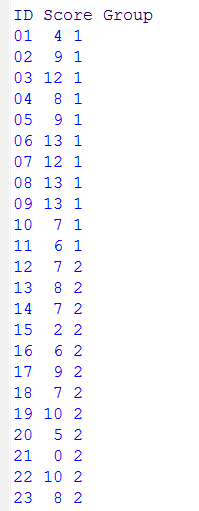
which contains the data for Table 7.7 in the text. Once you have entered your data and saved it, you can enter the command
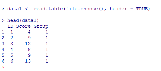
data1 <- read.table(file.choose(), header = TRUE)
The file.choose() command will cause it to open up a dialog box so that you can hunt around for the file you want. When you find it, just click on it and it will open and be known within R as data1. The header = TRUE command tells R that the first line contains variable names. Now rather than print out the whole file to see what we have, we can print
head(data1)
and get
Now you have your data read in, but perhaps not quite in the way you expect. One of your variables is named Score, but if you ask R to type out its values you will get
   > Score
   Error: object 'Score' not found
The problem (if there is one) is that data1 is what is called a data frame. A data frame is basically a file with a bunch of columns, and Score is part of that file. You could type "myData$Score" and everything would be fine, but putting "myData$" in front of each variable name is a pain. But if you type
   > attach(myData)
   > Score
    [1]  4  9 12  8  9 13 12 13 13  7  6  7  8  7  2  6  9  7 10  5  0 10  8
   >
then Score will be a legitimate variable by itself and you can now print it out as I did here. This is true whenever you have a data frame. You need to either use the "myData$subject" convention or attach the data frame. For these pages I will usually use the "attach()" command, but it is not without its problems. See my discussion of "attach()".
Suppose that you execute a program like this, perhaps make some changes, and then execute it again. You will get what looks like an error message (but isn't really). If I have a variable named Casenum sitting there, and then attach a data frame that also has a variable named "Casenum" in it, that copy of Casenum will mask (meaning hide) the prior variable named Casenum. If they are different, you may have a problem because you can't easily get to the old Casenum (unless you detach(data1)). Every time you run a program that attaches something, you will get a message like
The following object(s) are masked from 'lendata1 (position 3)':

ADDSC, CaseNum, Dropout, EngG, EngL, Gender, GPA, IQ, Repeat, SocProb
Most of the time that is not a problem because you are just masking the one variable with an exact copy. But the message will often lead you to think that you have made an error.
There are many other ways to enter data. One is by way of an Excel spreadsheet. Another is by way of the edit command. Try the following commands, one at a time, on the command line to see what happens.
   edit(data1)
   newfile <- edit(data.frame())
   write.table(data1, file = "Newfile.dat", row.names = FALSE)
The last command will create a file named Newfile.dat, but be sure to give it a more complete address or you won't know where it will end up. BUT having to type in the full search path is a pain. Assume that you have created a directory (folder) called "Learning-R." I don't care where you create it, but probably in your documents folder. Now go to the R console (where you have been seeing these results) and click on File/Change dir. Navigate to the Learning-R folder and click OK. Now that is your default directory, and if you just have 'file = "Newfile.dat"', it will be dumped in that directory. Much easier! That is also the first folder that will open if you use "file.choose()."
We are not limited to just printing out means. There are lots of other descriptive statistics that have their own functions. Some of these are shown below along with the results that R prints out.
   > mean(data4)
   [1] 2.6445

   > length(data4)  # reports the number of observations in data3.
   [1] 20

   > var(data4)
   [1] 0.4292892

   > sd(data4)
   [1] 0.6552017

   > hist(data4)
   >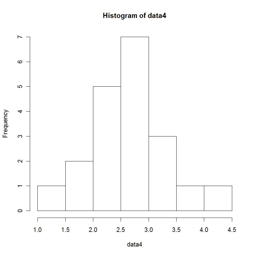
I cheated here a little bit. The graphic will not come out on your R console. It will come out in its own window. You may have to hunt around on your screen. Or go to the R icon on the bottom of your screen, click on it and select the image of the graphic.
Those few commands that you just saw will take you a long way. You could, for example, do many of the exercises in Chapter Two without learning any more. You could probably guess at a few other functions such as median(data4). Try typing sqrt(data4). I bet that isn't quite what you thought that you would get. I'll explain that in the next section.
dch