Computing Simple Effects in R and SPSS

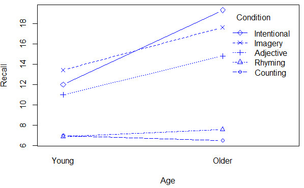
In the text I discuss the computation of simple effects in a factorial design. I think that simple effects can be very informative, there are different ways to compute them. One method is to run a separate analysis of variance at each level of the controlled fact and take the resulting F for each analysis as your test. That is a perfectly legitimate solution, but it loses power by using a reduced degrees of freedom for MS_error and it uses a less than optimal estimate of error. However when using standard software that is the easiest approach to take. The alternative approach is to calculate each F by using MS_error from the overall analysis of variance, along with its degrees of freedom. However, I don't know a simple way to compute the simple effects this way in either R or SPSS. So I have written R code that will do that, and that code can be found below. Although it is specifically related to the example in the text, a generalization to other examples should be straightforward. In addition, Andy Field (2009) has code for SPSS using the MANOVA procedure, which you probably have not seen. That syntax works just fine. That code is presented below, along with a graphic that shows that for the two conditions involving the least processing, age differences are nonexistent or trivial.

R Code

# This simple effects analysis is designed directly for the analysis of Eysenck's study.
# You can easily modify it to handle other kinds of data by changing the name of the
# data file and the names of variables. You could even modify it to handle higher order
# designs, but that would bring up questions of its own.

Eysenck.data <- read.table("http://www.uvm.edu/~dhowell/fundamentals9/DataFiles/Tab17-3.dat", header = TRUE)
names(Eysenck.data) 
k <- max(Eysenck.data$Condition)
l <- max(Eysenck.data$Age)
Eysenck.data$Condition <- factor(Eysenck.data$Condition)
Eysenck.data$Age <- factor(Eysenck.data$Age)
attach(Eysenck.data)
levels(Age) <- c("Young","Older")
levels(Condition) <- c("Counting", "Rhyming", "Adjective","Imagery","Intentional")
interaction.plot(x.factor = Age, trace.factor = Condition, response = Recall, fun = mean, 
type = "b", xlab = "Age", ylab = "Recall", col = "blue", pch = 1:5)
model.full <- lm(Recall ~ Age* Condition)      # All Effects
anova(model.full)
MS.error <- anova(model.full)$"Mean Sq"[4]
df.error <- anova(model.full)$Df[4]
cat("The simple effect of Condition at Age \n Age               F          df[error]         p \n")  
for (j in 1:l) {
     sub.data <- subset(Eysenck.data, Age == j)
     model.sub <- lm(Recall ~ Condition, data = sub.data)
     num <- (anova(model.sub))$"Mean Sq"[1] 
     F <- num/MS.error 
     p <- pf(F, k-1, df.error)
     cat("  ",j,"          ",F,"          ",df.error,"    ", 1 - p, "\n")}
cat("\n\n\n")
cat("The simple effect of Age at Condition  \n Condition        F           df[error]       p \n")
for (j in 1:k) {
  sub.data <- subset(Eysenck.data, Condition == j)
  model.sub <- lm(Recall ~ Age, data = sub.data)
  num <- (anova(model.sub))$"Mean Sq"[1] 
  F <- num/MS.error 
  p <- pf(F, k-1, df.error)
  cat("  ",j,"          ",F,"          ",df.error,"    ", 1 - p, "\n")

}

SPSS Code

The following code is modified from Field (2009) Discovering Statistics Using SPSS, 3rd ed. , Sage, page 442. I have added the command VS WITHIN to specify that I want the F values calculated by dividing by MS_within from the overall analysis. This is consistent with what I have said in the text and what I have done in R. (I hope that Andy doesn't mind.)

MANOVA   
Recall BY   Age(1 2)  Condition(1 5)
/DESIGN   Age WITHIN Condition(1) VS WITHIN     Age WITHIN Condition(2) VS WITHIN    
Age WITHIN Condition(3)VS WITHIN     Age WITHIN Condition(4) VS WITHIN  
Age WITHIN Condition(5)VS WITHIN
/DESIGN   Condition WITHIN Age(1) VS WITHIN     Condition WITHIN   Age(2) VS WITHIN   
/PRINT   
   CELLINFO   
   SIGNIF  (UNIV  AVERF   HF   GG   )