

Running a repeated measures analysis of variance in R can be a bit more difficult than running a standard between-subjects anova. This page is intended to simply show a number of different programs, varying in the number and type of variables. In another section I have gone to extend this to randomization tests with repeated measures, and you can find that page at www.uvm.edu/~dhowell/StatPages/R/RandomRepeatedMeasuresAnovaR.html
I should point out that there are a number of different ways of performing this analysis within R, and setting them up is not always obvious. But I strongly recommend that you do a search under "Repeated measures analysis of variance using R.
" I think that you will be surprised at the quality of the discussions you will find. I particularly like
The following example is loosely based on a study by Nolen-Hoeksema and
Morrow (1991). The authors had the good fortune to have measured depression in
college students two weeks before the Loma Prieta earthquake in California in
1987. After the earthquake they went back and tracked changes in depression in
these same students over time. The following example is based on their work, and
assumes that participants were assessed every three weeks for five measurement
sessions. I have changed the data from the ones that I have used elsewhere to build in
a violation of our standard assumption of sphericity. I have made measurements
close in time correlate highly, but measurements separated by 9 or 12 weeks
correlate less well. This is probably a very reasonable thing to expect, but it
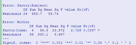
does violate our assumption of sphericity. If we ran a traditional repeated-measures analysis of variance on these data
we would find Notice that Fobt = 2.726, which is significant, based on
unadjusted df, with p = .034. Greenhouse and Geisser's correction
factor is 0.617, while Huynh and Feldt's is 0.693. Both of these lead to an
increase in the value of p, and neither is significant at α
= .05. (The F from a multivariate analysis of variance, which does not
require sphericity has p = .037.) Having two repeated measures is not really much different than having one. Instead of each subject's data across the one measure, we will randomize it across the second measure as well. For example, if we had a 2 X 5 design, both measures being repeated, each subject would have 10 scores and those 10 scores would be randomized. The data are taken from a study by Bouton and Swartzentruber (1985) on conditioned suppression, but I have only used the data from Group 2. (This study is discussed in my book on Statistical Methods for Psychologists, 8th ed.) on page 484ff. In this study each of 8 subjects was measured across two cycles on each of 4 phases, so Cycle and Phase are repeated measures. The code is shown below. I am going to use an example of a study with one between subject measure and one within subject measure, The data are from a study by King (1986) on motor activity in rats following the administration of midazolam under three different conditions. These data are from the same Bouten and Swartzentrub study used above. The difference is that I have used all three groups. Last revised: 6/26/2015
An example with 1 repeated measure
R Code for One Within Subject Variable
# R for repeated measures
# One within subject measure and no between subject measures
# Be sure to run this from the beginning because
# otherwise vectors become longer and longer.
library(car)
rm(list = ls())
## You want to clear out old variables --with "rm(list = ls())" --
## before building new ones.
data <- read.table("NolenHoeksema.dat", header = TRUE)
datLong <- reshape(data = data, varying = 2:6, v.names = "outcome", timevar
= "time", idvar = "Subject", ids = 1:9, direction = "long")
datLong$time <- factor(datLong$time)
datLong$Subject <- factor(datLong$Subject)
orderedTime <- datLong[order(datLong$time),]
options(contrasts=c("contr.sum","contr.poly"))
# Using "data = dataLong" I can use the simple names for the variables
modelAOV <- aov(outcome~factor(time)+Error(factor(Subject)), data = datLong)
print(summary(modelAOV))
obtF <- summary(modelAOV)$"Error: Within"[[1]][[4]][1]
par( mfrow = c(2,2))
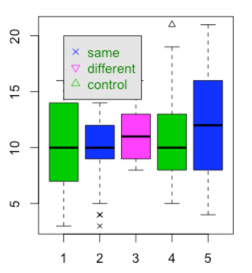
plot(datLong$time, datLong$outcome, pch = c(2,4,6), col = c(3,4,6))
legend(1, 20, c("same", "different", "control"), col = c(4,6,3),
text.col = "green4", pch = c(4, 6, 2),
bg = 'gray90')
The results follow.
- - - - - - - - - - - - - - - - - - - - - - - - - - - - -
 Error: factor(Subject)
Df Sum Sq Mean Sq F value Pr(>F)
Residuals 24 953.7 39.74
Error: Within
Df Sum Sq Mean Sq F value Pr(>F)
factor(time) 4 94.3 23.572 2.726 0.0337 *
Residuals 96 830.1 8.647
---
Signif. codes: 0 ‘***’ 0.001 ‘**’ 0.01 ‘*’ 0.05 ‘.’ 0.1 ‘ ’ 1
- - - - - - - - - - - - - - - - - - - - - - - - - - - - -
Error: factor(Subject)
Df Sum Sq Mean Sq F value Pr(>F)
Residuals 24 953.7 39.74
Error: Within
Df Sum Sq Mean Sq F value Pr(>F)
factor(time) 4 94.3 23.572 2.726 0.0337 *
Residuals 96 830.1 8.647
---
Signif. codes: 0 ‘***’ 0.001 ‘**’ 0.01 ‘*’ 0.05 ‘.’ 0.1 ‘ ’ 1
- - - - - - - - - - - - - - - - - - - - - - - - - - - - -
An example with two repeated measures
###  Test for Two Within-Subject Repeated Measures
  ### One tricky part of this code came from Ben Bauer at the Univ. of Trent, Canada.
  ### He writes code that is more R-like than I do. In fact, he knows more about R than
  ### I do.
# Two within subject variables, 1:8
# Data from Bouton & Schwartzentruber (1985) -- Group 2
# Methods8, p. 486

data <- read.table("Tab14-11long.dat", header = T)
n <- 8    #Subjects
cells <- 8    #cells = 2*4
nobs <- length(data$dv)
attach(data)
cat("Cell Means \n")
print(tapply(dv, list(Cycle,Phase), mean))    #cell means
cat("\n")
Subj <- factor(Subj)
Phase <- factor(Phase)
Cycle <- factor(Cycle)
   #Standard Anova
options(contrasts = c("contr.sum","contr.poly"))
model1 <- aov(dv ~ (Cycle*Phase) + Error(Subj/(Cycle*Phase)), contrasts = contr.sum)
summary(model1)   # Standard repeated measures anova
*** I have used this example elsewhere  except with a randomization approach.
# The resuts follow_____________________________________________________

Error: Subj
          Df Sum Sq Mean Sq F value Pr(>F)
Residuals  7   8411    1202

Error: Subj:Cycle
          Df Sum Sq Mean Sq F value Pr(>F)
Cycle      1  110.2  110.25   2.877  0.134
Residuals  7  268.2   38.32

Error: Subj:Phase
          Df Sum Sq Mean Sq F value Pr(>F)
Phase      3  283.4   94.46   1.029    0.4
Residuals 21 1928.1   91.82

Error: Subj:Cycle:Phase
            Df Sum Sq Mean Sq F value Pr(>F)
Cycle:Phase  3  147.6   49.21   0.728  0.547
Residuals   21 1418.9   67.57
One Between Subject Variable, One Within Subject Variable
.
# This code was originally written by Joshua Wiley, in the Psychology Department at UCLA.
# Modified for one between and one within for King.dat by dch
### Howell Table 14.4 ###
## Repeated Measures ANOVA with 2 variables
## Read in data, convert to 'long' format, and factor()
dat <- read.table("Tab14-4.dat", header = TRUE)
head(dat)
dat$subject <- factor(1:24)
datLong <- reshape(data = dat, varying = 2:7, v.names = "outcome", timevar
= "time", idvar = "subject", ids = 1:24, direction = "long")
datLong$Interval <- factor(rep(x = 1:6, each = 24), levels = 1:6, labels = 1:6)
datLong$Group <- factor(datLong$Group, levels = 1:3, labels = c("Control",
"Same", "Different"))
cat("Group Means","\n")
cat(tapply(datLong$outcome, datLong$Group, mean),"\n")
cat("\nInterval Means","\n")
cat(tapply(datLong$outcome, datLong$Interval, mean),"\n")
# Actual formula and calculation
King.aov <- aov(outcome ~ (Group*Interval) + Error(subject/(Interval)), data = datLong)
# Present the summary table (ANOVA source table)
print(summary(King.aov))
interaction.plot(datLong$Interval, factor(datLong$Group),
datLong$outcome, fun = mean, type="b", pch = c(2,4,6),
legend = "F",
col = c(3,4,6), ylab = "Mean of Outcome",
legend(4, 300, c("Same", "Different", "Control"), col = c(4,6,3),
text.col = "green4", lty = c(2, 1, 3), pch = c(4, 6, 2),
merge = TRUE, bg = 'gray90')
#The Results follow
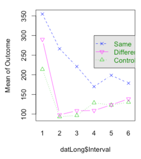 Error: subject
Df Sum Sq Mean Sq F value Pr(>F)
Group 2 285815 142908 7.801 0.00293 **
Residuals 21 384722 18320
Error: subject:Interval
Df Sum Sq Mean Sq F value Pr(>F)
Interval 5 399737 79947 29.852 < 2e-16 ***
Group:Interval 10 80820 8082 3.018 0.00216 **
Residuals 105 281199 2678
---
Error: subject
Df Sum Sq Mean Sq F value Pr(>F)
Group 2 285815 142908 7.801 0.00293 **
Residuals 21 384722 18320
Error: subject:Interval
Df Sum Sq Mean Sq F value Pr(>F)
Interval 5 399737 79947 29.852 < 2e-16 ***
Group:Interval 10 80820 8082 3.018 0.00216 **
Residuals 105 281199 2678
---
Two Between and One Within
# Two between subject variables, one within
# Data from St. Lawrence et al.(1995)
# Methods8, p. 479

#  Note: In data file each subject is called a Person, and I convert that to a factor.
#  In reshape, it creates a variable called "subject," but that is not what I want to use.
#  In aov the model is based on Person, not subject.
rm(list = ls())
data <- read.table("Tab14-7.dat", header = T)
head(data)
# Create factors
data$Condition <- factor(data$Condition)
data$Sex <- factor(data$Sex)
data$Person <- factor(data$Person)
#Reshape the data
dataLong <- reshape(data = data, varying = 4:7, v.names = "outcome", timevar
= "Time", idvar = "subject", ids = 1:40, direction = "long")
dataLong$Time <- factor(dataLong$Time)

tapply(dataLong$outcome, dataLong$Sex, mean)
tapply(dataLong$outcome, dataLong$Condition, mean)
tapply(dataLong$outcome, dataLong$Time, mean)
options(contrasts = c("contr.sum","contr.poly"))
model1 <- aov(outcome ~ (Condition*Sex*factor(Time)) + Error(Person/(Time)))
summary(model1)

# The results follow ________________________________
Error: Person
              Df Sum Sq Mean Sq F value Pr(>F)
Condition      1    107     107   0.215 0.6457
Sex            1   3358    3358   6.731 0.0136 *
Condition:Sex  1     64      64   0.128 0.7228
Residuals     36  17961     499
---
Error: Person:Time
                            Df Sum Sq Mean Sq F value Pr(>F)
factor(Time)                 3    274    91.4   0.896 0.4456
Condition:factor(Time)       3   1378   459.3   4.507 0.0051 **
Sex:factor(Time)             3    780   260.0   2.551 0.0594 .
Condition:Sex:factor(Time)   3    476   158.8   1.558 0.2037
Residuals                  108  11006   101.9
...
Two Within-Subject Repeated Measures
and One Between-subjects Measure
rm(list = ls())
data <- read.table("Tab14-11.dat", header = T)
attach(data)
Phase <- factor(rep(1:2, each = 24, times = 4))
Cycle <- factor(rep(1:4, each = 48))
Group = factor(rep(1:3, each = 8,times = 8))
dv <- c(C1P1, C1P2, C2P1, C2P2, C3P1, C3P2, C4P1, C4P2)
Subj <- factor(rep(1:24, times = 8))
n <- 24    #Subjects
withincells <- 8    #withincells = 2*4
nobs <- length(dv)

cat("Cell Means Across Subjects \n")
print(tapply(dv, list(Cycle,Phase), mean))    #cell means
cat("\n")
#Standard Anova
options(contrasts = c("contr.sum","contr.poly"))
model1 <- aov(dv ~ (Group*Cycle*Phase) + Error(Subj/(Cycle*Phase)),
  contrasts = contr.sum)
print(summary(model1))   # Standard repeated measures anova
# The results follow
Error: Subj
          Df Sum Sq Mean Sq F value Pr(>F)
Group      2   4617  2308.4   3.083  0.067 .
Residuals 21  15723   748.7
---
Signif. codes:  0 ‘***’ 0.001 ‘**’ 0.01 ‘*’ 0.05 ‘.’ 0.1 ‘ ’ 1

Error: Subj:Cycle
            Df Sum Sq Mean Sq F value   Pr(>F)
Cycle        3   2727   909.0  12.027 2.53e-06 ***
Group:Cycle  6   1047   174.5   2.309   0.0445 *
Residuals   63   4761    75.6
---
Signif. codes:  0 ‘***’ 0.001 ‘**’ 0.01 ‘*’ 0.05 ‘.’ 0.1 ‘ ’ 1

Error: Subj:Phase
            Df Sum Sq Mean Sq F value   Pr(>F)
Phase        1  11703   11703  129.85 1.88e-10 ***
Group:Phase  2   4054    2027   22.49 6.01e-06 ***
Residuals   21   1893      90
---
Signif. codes:  0 ‘***’ 0.001 ‘**’ 0.01 ‘*’ 0.05 ‘.’ 0.1 ‘ ’ 1

Error: Subj:Cycle:Phase
                  Df Sum Sq Mean Sq F value  Pr(>F)
Cycle:Phase        3    742  247.17   4.035 0.01090 *
Group:Cycle:Phase  6   1274  212.30   3.466 0.00505 **
Residuals         63   3859   61.26
---
Signif. codes:  0 ‘***’ 0.001 ‘**’ 0.01 ‘*’ 0.05 ‘.’ 0.1 ‘ ’ 1