For this page I will work through an example for each of the traditional nonparametric tests. I will give one example of each, using the examples or exercises in Chapter 20.
I will take the data from McConaughy (1990) on the number of inferences produced by younger and older children. The code is shown below. In this code I specify "exact = TRUE" so that R does not use an approximation. With so few data points, it is very simple to compute the exact probability. I also specified that "alternative = "less", because we fully expect the younger children to show fewer inferences. You can see that the difference is statistically significant. We would obtain very similar results if we used a standard t test
### Wilcoxon-Mann-Whitney Rank Sum test
inference <- c(12, 4, 8, 10, 2, 22, 20, 6, 24, 14, 26, 18, 16, 28)
AgeGrp <- rep(c(1,2), each = 7)
wilcox.test(inference ~ AgeGrp, alternative = "less", paired = FALSE, exact = TRUE)
- - - - - - - - - - - - - - - - - - - - - -
	Wilcoxon rank sum test

data:  inference by AgeGrp
W = 11, p-value = 0.04866
alternative hypothesis: true location shift is less than 0
When we move to the situation with paired samples, we need to use a different test created by Wilcoxon. This test basically asks if the ranks of the differences are more positive (or more negative) than would be expected. I will use the data that appear in Exercise 20.18, which asks if the volume of the left hippocampus in schizophrenic adults is larger or smaller than the same volume for their identical twin. It was assumed that the volume would be lower in the schizophrenic twin.
wilcox.test(x = normal, y = schizophrenic, alternative = "greater", paired = TRUE,
 exact = TRUE)
- - - - - - - - - - - - - - - - - - - - - - - - - - - -
	Wilcoxon signed rank test

data:  normal and schizophrenic
	Wilcoxon signed rank test

data:  normal and schizophrenic
V = 111, p-value = 0.001007
alternative hypothesis: true location shift is greater than 0
Notice that I have done something different here. I ran the standard Kruskal-Wallis test on the three groups, and found a significant difference (p = .034). I then wanted to compare the first two groups combined with the third group. The normal way to do this would be to go back to a rank-sum test, but I also used the Kruskal-Wallis with two groups, which is perfectly legitimate. Notice that for both of those tests the difference was significant, with nearly equal probabilities.
The last traditional nonparametric test that I will examine is Friedman's test. For this I will use the data in Exercise 20.14 on truancy before, during, and after a stay in a group home. The data are found in that exercise.
I had trouble running this test until I looked in Field's Discovering Statistics Using R (2012). Field said "We can do Friedman's ANOVA using the friedman.test() function. This function is a bit of a prima donna because, in order to work it demands that (1) you give it a matrix rather than a data frane, because according to Andy, it thinks that dataframes smell like rotting brains, and (2) it wants all of the variables of interest in one data set, and there mustn't be any additional variables." (Well, Andy is always fun to read!). So I put it in a matrix and it worked, though the help screen does not say that you need to do this.
###	Friedman rank sum test
data <- matrix(c(10, 5, 8, 12, 8, 7, 12, 13, 10, 19, 10, 12, 5, 10, 8, 13, 8, 7, 20,
 16, 12, 8, 4, 5, 12, 14, 9, 10, 3, 5, 8, 3, 3, 18, 16, 2), byrow = TRUE, ncol = 3)
friedman.test(data)
- - - - - - - - - - - - - - - - - - - - - - - - -
data:  data
Friedman chi-squared = 9.234, df = 2, p-value = 0.009882
From the printout you can see that the difference is significant, although I would question the idea of reporting the probability to six significant digits when you are using the chi-square distribution as an approximation.
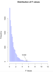
In the text I wrote about randomization tests and said that the code would be on the web. Here is the code. Notice that I have taken a set of data and calculated F, which I stored away as Fobt. If there are no effects due to groups, a data point could fall in any one of the three groups. So I replicate the design 10,000 times, each time randomly assigning the scores to the groups and calculating an F value. When I am done I have a distribution of 10,000 F's obtained when there are no treatment effects. I can then compare the F that I obtained from the real data to that distribution. Finally, I drew a histogram of those F values.
### Randomization test on maternal adaptation


matadapt <- read.table("http://www.uvm.edu/~dhowell/fundamentals9/DataFiles/Tab16-6.dat",
 header = TRUE)
head(matadapt)
attach(matadapt)
## Calculate the obtaiend F for these data
Group <- factor(Group)    # Don't forget to do this for factors
model.1 <- lm(Adapt ~ Group)
result <- anova(model.1)
Fobt <- result$"F value"[1]    # This just extracts the F from the original analysis

nreps = 10000
k = length(Adapt)         # How many scores are there?
Fs <- numeric(nreps)      # Set aside space for 1000 F values under the null
for (i in 1:nreps)  {     # Do this stuff nreps times}
   newAdapt <- sample(Adapt, size = k, replace = FALSE) # randomize the dep. var.
   model.2 <- lm(newAdapt ~ Group)                      # Rerun anova with randomized data
   Fs[i] <- anova(model.2)$"F value"[1]                 # Collect all 1000 Fs
}
Fsort <- sort(Fs)
prob <- length(Fs[Fs >= Fobt])/nreps
cutoff <- Fsort[nreps*.95]
cat(" 5 percent of the F values exceed ",cutoff)
cat("The actual probability from randomization is ", prob)
hist(Fs, breaks = 50, xlab = "F Values", main = "Distribution of F values",
 density = 10, col = "blue")
F <- round(Fobt, digits = 3)
legend(3, 200, F, bty = "n")
arrows(4, 90, 5.53, 5)