

A factorial analysis of variance is quite straight-forward in R as long as we have equal sample sizes. Things do get a bit messy if the sample sizes are unequal, and I will touch on that very briefly in the code below. I will use the data from Table 17.3 as an example. It represents a 2 X 5 analysis of variance.
As with the one-way analysis of variance, we will use the linear model (lm()) command with the independent variables specified as factors. We will then use the anova() function to print out the results we want. This is true of all analyses of variance. We first generate a model using lm(), with independent variables as factors, and then we use another function to extract the information we seek. Our code is given below.
rm(list = ls())
data2 <- read.table("http://www.uvm.edu/~dhowell/fundamentals9/DataFiles/Tab17-3.dat",
 header = TRUE)
attach(data2)
Age <- factor(Age)
Condition <- factor(Condition)
model2 <- lm(Recall ~ Age * Condition)
anova(model2)
#____________________________________
Analysis of Variance Table

Response: Recall
                   Df      Sum Sq   Mean Sq   F value   Pr(>F)
Age                1        240.2     240.2   29.936   3.98e-07 ***
Condition          4       1514.9     378.7   47.191    < 2e-16 ***
Age:Condition      4        190.3      47.6    5.928   0.000279 ***
Residuals         90        722.3       8.0
Notice that the first line of code contained "rm(list = ls())." You should probably always do that. Every once in a while you have a variable hanging on from a previous analysis, and it has the same name as one of your new variables. It is very easy to obtain some weird answers when that happens.
Notice that I converted my independent variables to factors. In the lm() statement I first put the dependent variable, followed by "~", followed by Age * Condition. That tells R that I want the main effect of Age, the main effect of Condition, and their interaction. I could have accomplished the same thing by Recall ~ Age + Condition + Age*Condition."
The first thing that I do when I have the anova function print out the summary table is to check the degrees of freedom. If you have messed up somewhere, there is a high likelihood that the degrees of freedom will be wrong. The most obvious error is to forget to specify that the independent variables are factors. If you make that error, the degrees of freedom for each effect will be 1 rather than k - 1.
The analysis gave me what I would expect. There is a significant effect for Age, for Condition, and, most importantly, for the interaction. We can plot that interaction by simply using the interaction.plot() function. I show this below.Clearly the mean of the younger participants increases more rapidly across conditions tha the mean of the older participants.
interaction.plot(x.factor = Condition, trace.factor = Age, response = Recall, fun = mean,
type = "l")

The plot follows: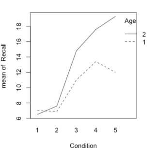
If we want to look at the simple effects--e.g. the Condition effect at each level of Age, we simply create subsets of the data. I show this for only the older subjects, whose Age is coded as 1. But you will note that if you compare this result to the one in the text, there is a difference. Namely, the F value is somewhat different and, most importantly, we only have 45 degrees of freedom for the error term. This is caused by the fact that the data are literally cut in half and the error term for each half is used. In the text I took the error term from the factorial analysis, which had 90 degrees of freedom, and used that. If you want to do the same, you will need to do it by hand. I don't know a way to tell R to do that. But it's pretty easy to do that division. For example, 87.88/8.0 = 10.98, which is within rounding error of the result in the text.
model3 <- lm(Recall[Age == 1] ~ Condition[Age == 1])
anova(model3)
#__________________________
Analysis of Variance Table

Response: Recall[Age == 1]
                    Df Sum Sq Mean Sq F value   Pr(>F)
Condition[Age == 1]  4  351.5   87.88   9.085 1.82e-05 ***
Residuals           45  435.3    9.67
In the text I cover effect size measures for both correlational measures and standardized distance measures. For many problems in the analysis of variance with multiple groups it makes sense to use eta-squared or omega-squared because they involve all of the levels of an independent variable. I will use the example of Eysenck's study, focusing on the difference between the five conditions. I will use the overall main effect for Condition, although I could work with the simple effects equally well.
First I will do it the pencil and paper way. I find the appropriate sum of squares from the printout and then manually do the calculations. If you are only going to do this once in a while, that is probably the easiest. But there is another way, and one that teaches us a bit about objects. I show that next.
As I have said previously, when R computes the analysis, it stores a whole bunch of stuff away in an object, here called model2. When you ask for the summary table, it does some more calculations and stores that away in an object called anova(model2). If you type "names(anova(model2))" you will see " [1]"Df" "Sum Sq" "Mean Sq" "F value" "pr(>F)". Each of those is a list of values. I can type "print(anova(model2)$"Sum Sq")" and get "[1] 240.25 1514.94 190.30 722.30," which are the appropriate sums of squares. For example, if I type "SStot <- sum((anova(model2)$"Sum Sq"), I have the total sum of squares (2667.79). Then for SScond I can enter "SScond <- anova(model2)$"Sum Sq"[2]. The "[2]" there asks for the second element of that vector. Now I can compute "eta-sq.Condition <- SStot/SScond.
rm(list = ls())
data2 <- read.table("http://www.uvm.edu/~dhowell/fundamentals9/DataFiles/Tab17-3.dat",
                    header = TRUE)
attach(data2)
Age <- factor(Age)
Condition <- factor(Condition)
model2 <- lm(Recall ~ Age * Condition)
anova(model2)
names(anova(model2))
SStot <- sum(anova(model2)$"Sum Sq")
SScond <- anova(model2)$"Sum Sq"[2]
etaSq.Condition <- SScond/SStot
MSerror <- anova(model2)$"Mean Sq"[4]
DFcond <- anova(model2)$"Df"[2]
omegaSq.Condition <- (SScond - DFcond*MSerror)/(SStot + MSerror)
cat("Eta Square for Condition - ", etaSq.Condition)
cat("Omega Square for Condition - ", omegaSq.Condition)
#______________________________________________
> cat("Eta Square for Condition - ", etaSq.Condition)
Eta Square for Condition =  0.5678633
> cat("Omega Square for Condition - ", omegaSq.Condition)
Omega Square for Condition =  0.5541629
That is a very brief introduction to the use of objects and lists within objects. You can extract all sorts of specific elements from those objects, but it sometimes takes a good bit of trial and error to get the element you want. I don't expect that any student will memorize this approach, but it is here if you need it.
I won't go into calculating a d type measure because we saw that in the last chapter and you should be able to generalize from there.
Running a factorial analysis of variance with unequal sample sizes is not quite as easy as you might think. You could run it the same way that we did above, but the sum of squares that you obtain are most likely not the sum of squares you want. Now the people who created R would strongly disagree with me in what follows, but I think that I have most of the people in the behavior sciences on my side. When we have equal sample sizes, the effects are independent of one another. So that you can look at the effect of Condition without adjusting for Age and the Condition x Age interaction. Similarly for the other effects. But with unequal n's the effects are not independent. So what do you do to adjust the effect of Condition for Age and the interaction? That is what the fight is about. The R folks want you to do what I have done above, but that means that we will obtain the complete effect of Age, then the effect of Condition adjusted for Age, and then the interaction adjusted for Age and Condition. For what behavioral scientists do, that doesn't usually make sense.
SPSS does things differently. It adjusts each effect for the other effects. This is called a Type III analysis, and R people love to sneer at it. But that is the analysis that I will suggest that you do. However, you can't run that analysis from the base package of R. Well you can, but it is messy. But John Fox came to the rescue. He created a package called "car." (That stands for the title of his book (Companion to Applied Regression.) Fox allows you to do it the R way, called Type I, or to adjust the interaction for the main effects and then the main effects for only each other (Type II), or each effect adjusted for all other effects (Type III).
To use Fox's package, install and load "car." Then follow the code that I have above, but instead of using "anova(model2)", use "Anova(model2)". The only difference is that Anova is capitalized. The little bit of code is shown below. Note that it is important to set the type of contrasts for Age and Condition. You can see how I have done that in the code. I definitely do not want to go into that discussion. In fact, I would go so far as to suggest that it would be easier to run the analysis in SPSS. Much as I like R, it is easy to make a mistake and have the wrong analysis.
library(car)
contrasts(Age) <- contr.sum(2)
contrasts(Condition) <- contr.sum(5)
model2 <- lm(Recall ~ Age * Condition)
Anova(model2, type = "III")
I will take only one example from the exercises because it is similar to many of the others. This is a case where I can reasonably enter the data by hand rather than reading it from a data file. The data and the analysis are shown below.
# Exercise 17.17
rm(list = ls())  #We had Age in the previous example, and I don't want confusion
Age <-factor(rep(c(1,2), each = 20) )
Level <- factor(rep(c(1,2,1,2), each = 10))
dv <- c(8,6,4,6,7,6,5,7,9,7,21,19,17,15,22,16,22,22,18,21,
        9,8,6,8,10,4,6,5,7,7,10,19,14,5,10,11,14,15,11,11)
model4 <- lm(dv ~ Age * Level)
anova(model4)