1/3 1/3 1/3 -1/2 -1/2 1/2 1/2 -1 0 0 1 -1 0 0 0 0 0 0 1 -1


This page was originally created to correct an error that I included as the answer to one of my exercises in an earlier edition of Statistical Methods for Psychology, 7th edition. (I want to thank David Morse at Mississippi State for pointing the problem out to me.) That book is now out of date, but the issue that was raised applies generally and is certainly not restricted to users of my texts. The question of handling an analysis of variance with unequal sample sizes deserves attention. Hence, this page.
When you have a design with equal samples sizes (called a balanced design) it doesn't matter if you get the mean of two groups by adding up all of their scores and dividing by the number of scores, or if you just average their means. For example, if we have
Group 1 5 6 7 9 10 sum = 37, mean = 37/5 = 7.4
Group 2 8 9 12 7 14 sum = 50, mean = 50/5 = 10
Combined scores Mean = (5 + 6 + 7 + 9 + 10 + 8 + 9 + 12 + 7 + 14)/10
= (37 + 50)/10 = 87/10 = 8.7
Average mean Mean = (7.4 + 10)/2 = 17.4/2 = 8.7
You can use a formula that is based on the totals of the groups or on the means of the groups and you will come out at the same place with the same answer.
But when you have an unbalanced design there can be a very large difference.
Group 1 5 6 sum = 11, mean = 11/2 = 5.5
Group 2 8 9 12 7 14 sum = 50, mean = 50/5 = 10
Combined scores Mean = (5 + 6 + 8 + 9 + 12 + 7 + 14)/7
= (11 + 50)/7 = 61/7 = 8.71 weighted mean
Average mean Mean = (5.5 + 10)/2 = 15.5/2 = 7.75 unweighted mean
Notice that those two calculations lead to different answers, and their difference will usually increase as the difference in sample sizes increases. The weighted mean with unequal n's is more heavily influenced by the larger size of Group 2, which pulls the combined mean closer to the mean of that group. For the unweighted mean the groups are weighted equally, regardless of sample size, and the combined mean falls half way between the two group means. This may be a bit clearer if I recalculate the mean resulting from lumping all the scores together as
Combined groups Mean = (5 + 6 + 8 + 9 + 12 + 7 + 14)/7 = (2*11 + 5*50)/7 = 61/7 = 8.71
= n1X̄1 + n2X̄2/(n1 + n2) = (2*5.5 + 5*10)/7 = 61/7 = 8.71Here you can see that this approach explicitly weights the means by the sample sizes, giving more weight to the mean based on a larger sample. This is called the "weighted means" approach. The other approach treats the means equally, and is often known as an "unweighted" or "equally weighted means" solution or the least squares solution.
Consider the following data on five groups.
Group 1       8.706 10.362 11.552 6.941 10.983 10.092 6.421 14.943   Mean = 10, sd = 7.4  n = 8
Group 2       15.931 22.968 18.590 16.567 15.944                     Mean = 18, sd = 8.9, n = 5
Group 3       21.637 14.49217.965 18.851 22.891 22.028 16.884 17.252 Mean = 19, sd = 8.6, n = 8
Group 4       18.325 25.435 19.141 21.238 22.196 18.038 22.628       Mean = 21, sd = 7.2, n = 7
Group 5       31.163 26.053 24.419 32.145 28.966 30.207 29.142
              33.212 25.694                                          Mean = 29, sd = 9.3, n = 9
I am presenting the unweighted means solution, because I can think of relatively few times that we would want to pay more attention to one group than another if we are trying to compare group means. It is based on means rather than totals and uses the appropriate denominator to handle the unequal sample sizes.
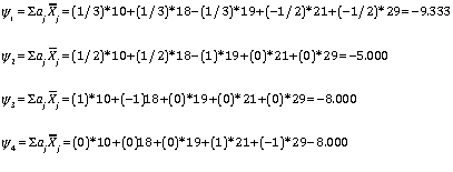
Assume that we have the following set of contrasts that we want to run. We want to compare the first three groups with the last two, The first two with the third, the first with the second, and the third with the fourth. The following set of contrasts coefficients will give us those contrasts. Below the coefficients you will see the computation of the linear contrasts. You can see that each of them represents the difference between the means of the two "sets" in each contrast. Notice that these contrasts are orthogonal.
	 1/3    1/3    1/3    -1/2    -1/2
	 1/2    1/2     -1     0        0
	  1      -1      0     0        0
	  0       0      0     1       -1
Below I give the answer for the first contrast. It is 9.333. Using the above formula, the other contrasts will come out to be (10+18)/2-18 = -5, (10-18) = -8, and (21-29) = -8.
This approach is the one that I prefer unless there are good reasons to weight means differently. But what if we do want to weight them differently because the sample sizes clearly reflect something about population sizes?
To run this analysis using R you can use the following code. I show the solution following the code.
rm(list = ls())
dv <- c(8.706, 10.362, 11.552,  6.941, 10.983, 10.092,  6.421, 14.943, 15.931, 22.968,
 18.590, 16.567, 15.944, 21.637, 14.492, 17.965, 18.851, 22.891, 22.028, 16.884, 17.252,
 18.325, 25.435, 19.141, 21.238, 22.196, 18.038, 22.628, 31.163, 26.053, 24.419, 32.145,
 28.966, 30.207, 29.142, 33.212, 25.694)
group <- rep(1:5, c(8,5,8,7,9)
group <- factor(group)
L <- matrix(c(1,1,1,1,1,.333, .333, .333, -.5, -.5,
 1/2, 1/2, -1, 0, 0,
 1, -1, 0, 0, 0,
 0, 0, 0,  1, -1), byrow = TRUE, nrow = 5)
Linv <- solve(L)                              # Take the inverse of L)
new.contrasts <- Linv[,-1]                    # Strip out the first column of L
contrasts(group) <- new.contrasts             # Set the contrasts equal to the ones in Linv)
model1 <- lm(dv ~ group)
summary(model1,split=list(group = list("First 3 vs last 2"= 1, "One and Two vs Three" = 2,
 "One vs Two" = 3, "Four vs Five" = 4)))

___________________________________________________________________________

Analysis of Variance Table

Response: dv
          Df  Sum Sq Mean Sq F value    Pr(>F)
group      4 1561.32  390.33  47.104 5.717e-13 ***
Residuals 32  265.17    8.29
---


Coefficients:
            Estimate Std. Error t value Pr(>|t|)
(Intercept)  19.4001     0.4831  40.161  < 2e-16 ***
group1       -9.3297     0.9694  -9.624 5.74e-11 ***
group2       -5.0000     1.3073  -3.825 0.000572 ***
group3       -8.0000     1.6411  -4.875 2.86e-05 ***
group4       -8.0000     1.4507  -5.515 4.44e-06 ***
---


Residual standard error: 2.879 on 32 degrees of freedom
Multiple R-squared:  0.8548,	Adjusted R-squared:  0.8367
F-statistic:  47.1 on 4 and 32 DF,  p-value: 5.717e-13
Notice that there are two parts of the printout. The part given by "anova(model1)" is the standard analysis of variance summary table. It is clear that the difference is statistically significant. The part given by "summary(model1) gives us the results obtained by applying the appropriate coefficients. Notice that the intercept is the grand mean, the coefficient labelled "group1" is the result of applying the first set of coefficients to the means, similarly for the next three rows. Notice also that we have a t test on each of these contrasts and they are all significant. You can see that these are the same results I calculated above.
What is important in the R code is that we take the original matrix of coefficients and compute its inverse. R refers to the inverse as "solve." If you were running SPSS or SAS, you would not do that because it is built into the program. In other words, SPSS takes its own inverse automatically. But R does not do things that way.
If you failed to compute the inverse and just used the matrix you entered, you would find an odd result. It would look like
Coefficients:
            Estimate Std. Error t value Pr(>|t|)
(Intercept)  19.3978     0.4831  40.155  < 2e-16 ***
group1      -11.2046     1.1642  -9.624 5.74e-11 ***
group2       -3.3333     0.8716  -3.825 0.000572 ***
group3       -4.0000     0.8205  -4.875 2.86e-05 ***
group4       -4.0000     0.7253  -5.515 4.44e-06 ***
Other than the intercept, these coefficients look like nothing you have seen before. I can't even figure out how they were calculated. But, if you notice, the t values are the same that we found above. Curious!!!
If we run the same analysis using SPSS, we obtain the following printout. These are the same results that we obtained using R, which is comforting. You might notice the little footnote. It complains that the sum of the coefficients is not = 0, but you can see that I supplied the right coefficients. Apparently it is annoyed that .999 is not equal to 1.0. But they don't allow me to supply more digits.

 dch
dch