
![]()
![]()
As of the time of this writing, I will restrict my discussion to designs with one repeated measurement, and no between-subjects measures. I will work at expanding the coverage later, when I write the necessary procedures. I do show the code for the traditional parametric analysis of variance for several other designs at the very end of this document. You might take the code I have here, modify it for the more complex designs, and see if you can get it to run.
Just as we did with the one-way analysis of variance on independent samples, we will use the normal F statistic. It summarizes the differences between means, and eliminates the effects of between-subjects variability.
With repeated measures, we want to permute the data within a subject, and we don't care about between-subject variability. If there is no effect of treatments or time, then the set of scores from any one participant can be exchanged across treatments or time. In what follows I will assume that the repeated measure is over time, though there is no restriction that it need be.
The following example is loosely based on a study by Nolen-Hoeksema and Morrow (1991). The authors had the good fortune to have measured depression in college students two weeks before the Loma Prieta earthquake in California in 1987. After the earthquake they went back and tracked changes in depression in these same students over time. The following example is based on their work, and assumes that participants were assessed every three weeks for five measurement sessions.
I have changed the data from the ones that I have used elsewhere to build in a violation of our standard assumption of sphericity. I have made measurements close in time correlate highly, but measurements separated by 9 or 12 weeks correlate less well. This is probably a very reasonable thing to expect, but it does violate our assumption of sphericity.
If we ran a traditional repeated-measures analysis of variance on these data we would find
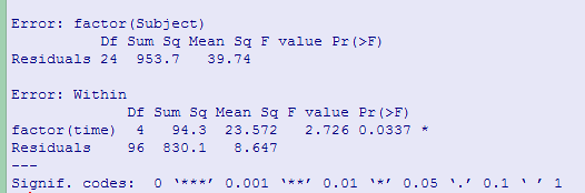
Notice that Fobt = 2.726, which is significant, based on unadjusted df, with p = .034. Greenhouse and Geisser's correction factor is 0.617, while Huynh and Feldt's is 0.693. Both of these lead to an increase in the value of p, and neither is significant at a = .05. (The F from a multivariate analysis of variance, which does not require sphericity has p = .037.)
We can apply a randomization test to these data using the code shown below. This code may be harder to read than most. That is because I had a lot of trouble coming up with a way of randomizing the time measurements within subjects. I finally did it, but it takes a bit of thinking. The code also produces a standard analysis of variance table. The "Error: factor(Subject)" section just tells you about the variability among subjects, which is not particularly interesting. The "Error:Within" section tests the time (or trials) factor and is what we mainly want.
#  R for repeated measures
#  One within subject measure and no between subject measures
#  Be sure to run this from the beginning because otherwise vectors become longer and longer.
library(car)
rm(list = ls())
  ##  You want to clear out old variables -with "rm(list = ls())" - before building new ones.
data <- read.table(("http://www.uvm.edu/~dhowell/StatPages/ResamplingWithR/RandomRepeatMeas/NolenHoeksema.dat"), header = TRUE)

datLong <- reshape(data = data, varying = 2:6, v.names = "outcome", timevar
= "time", idvar = "Subject", ids = 1:9, direction = "long")

datLong$time <- factor(datLong$time)
datLong$Subject <- factor(datLong$Subject)
orderedTime <- datLong[order(datLong$time),]
options(contrasts=c("contr.sum","contr.poly"))
modelAOV <- aov(outcome~factor(time)+Error(factor(Subject)), data = datLong)
print(summary(modelAOV))
obtF <- summary(modelAOV)$"Error: Within"[[1]][[4]][1]

par( mfrow = c(2,2))
plot(datLong$time, datLong$outcome, pch = c(2,4,6), col = c(3,4,6))
legend(1, 20, c("same", "different", "control"), col = c(4,6,3),
                      text.col = "green4",  pch = c(4, 6, 2),
                       bg = 'gray90')
nreps <- 1000
counter <- 0
Fsamp <- numeric(nreps)

times <- c(1:5)
permTimes <-NULL

for (i in 1:nreps) {
for (j in 1:25) {
  permTimes <- c(permTimes, sample(times,5,replace = FALSE))
  }
orderedTime$permTime <- permTimes
sampAOV <- aov(outcome~factor(permTime)+Error(factor(Subject)), data = orderedTime)
Fsamp[i] <- summary(sampAOV)$"Error: Within"[[1]][[4]][1]
if (Fsamp[i] > obtF) counter = counter + 1
permTimes <- NULL
}

p <- counter/nreps
cat("The probability of sampled F greater than obtained F is = ", p, '\n')
 hist(Fsamp, breaks = 50, bty = "n")
 legend(1.5,50,bquote(paste(p  == .(p))), bty = "n" )
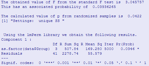
Notice that our sample F is the same, as it should be, and the associated p is .033. This agrees closely with the unadjusted p value for the F. It does not agree, however, with either of the adjusted p values (not shown). Here we have a situation where the p computed from the randomization test would allow us to reject the null hypothesis of no difference, but the p computed from the appropriate adjustment of Greenhouse and Geisser would not allow rejection.
################################################################################# This was written by Joshua Wiley, in the Psychology Department at UCLA. # Modified for one between and one within for King.dat by dch ### Howell Table 14.4 ### ## Repeated Measures ANOVA with 2 variables ## Read in data, convert to 'long' format, and factor() dat <- read.table("http://www.uvm.edu/~dhowell/methods8/DataFiles/Tab14-4.dat", header = TRUE) head(dat) dat$subject <- factor(1:24) datLong <- reshape(data = dat, varying = 2:7, v.names = "outcome", timevar = "time", idvar = "subject", ids = 1:24, direction = "long") datLong$Interval <- factor(rep(x = 1:6, each = 24), levels = 1:6, labels = 1:6) datLong$Group <- factor(datLong$Group, levels = 1:3, labels = c("Control", "Same", "Different")) cat("Group Means","\n") cat(tapply(datLong$outcome, datLong$Group, mean),"\n") cat("\nInterval Means","\n") cat(tapply(datLong$outcome, datLong$Interval, mean),"\n") # Actual formula and calculation King.aov <- aov(outcome ~ (Group*Interval) + Error(subject/(Interval)), data = datLong) # Present the summary table (ANOVA source table) print(summary(King.aov)) interaction.plot(datLong$Interval, factor(datLong$Group), datLong$outcome, fun = mean, type="b", pch = c(2,4,6), legend = "F", col = c(3,4,6), ylab = "Mean of Outcome",) legend(4, 300, c("Same", "Different", "Control"), col = c(4,6,3), text.col = "green4", lty = c(2, 1, 3), pch = c(4, 6, 2), merge = TRUE, bg = 'gray90')
################################################################################# Two within subject variables, one between # Data from Bouton & Schwartzentruber (1985) # Methods8, p. 486 rm(list = ls()) data <- read.table("http://www.uvm.edu/~dhowell/methods8/DataFiles/Tab14-11.dat", header = T) attach(data) ## I should use "reshape," but I can't get it to work. This is pretty easy. Phase <- factor(rep(1:2, each = 24, times = 4)) Cycle <- factor(rep(1:4, each = 48)) Group = factor(rep(1:3, each = 8,times = 8)) dv <- c(C1P1, C1P2, C2P1, C2P2, C3P1, C3P2, C4P1, C4P2) Subj <- factor(rep(1:24, times = 8)) cat("Means and sd by Group \n") tapply(dv, Group, mean); tapply(dv, Group, sd) cat("\n Means and sd by Cycle\n") tapply(dv, Cycle, mean); tapply(dv, Cycle, sd) cat("\n Means and sd by Phase\n") tapply(dv, Phase, mean); tapply(dv, Phase, sd) options(contrasts = c("contr.sum","contr.poly")) model1 <- aov(dv ~ (Group*Cycle*Phase) + Error(Subj/(Cycle*Phase)), contrasts = contr.sum) print(summary(model1)) print(coefficients(model1)) # This will give mean deviations) library(ez) # Alternative approach using ezANOVA df <- data.frame(cbind(Subj, dv, Group, Phase, Cycle)) df$Group <- factor(df$Group) df$Phase <- factor(df$Phase) df$Cycle <- factor(df$Cycle) df$Subj <- factor(df$Subj) modelez <- ezANOVA(data <- df, dv = dv, wid = Subj, within = .(Phase, Cycle), between = Group, ,type = 3 ) print(modelez) #ges = Generalized Eta Square, GGE - Greenhouse and Geisser, HFe = Huynh * Feldt) # I get slightly different values for the Greenhouse & Geisser and the #Huynh & Feldt correction
################################################################################# Two between subject variables, one within # Data from St. Lawrence et al.(1995) # Methods8, p. 479 # Note: In data file each subject is called a Person, and I convert that to a factor. # In reshape, it creates a variable called "subject," but that is not what I want to use. # In aov the model is based on Person, not subject. rm(list = ls()) data <- read.table("http://www.uvm.edu/~dhowell/methods8/DataFiles/Tab14-7.dat", header = T) head(data) # Create factors data$Condition <- factor(data$Condition) data$Sex <- factor(data$Sex) data$Person <- factor(data$Person) #Reshape the data dataLong <- reshape(data = data, varying = 4:7, v.names = "outcome", timevar = "Time", idvar = "subject", ids = 1:40, direction = "long") dataLong$Time <- factor(dataLong$Time) tapply(dataLong$outcome, dataLong$Sex, mean) tapply(dataLong$outcome, dataLong$Condition, mean) tapply(dataLong$outcome, dataLong$Time, mean) options(contrasts = c("contr.sum","contr.poly")) model1 <- aov(dataLong$outcome ~ (dataLong$Condition*dataLong$Sex*factor(dataLong$Time)) + Error(dataLong$Person/(dataLong$Time))) summary(model1)
![]()
![]()
Last revised: 12/9/2013