Bootstrapping Two Medians

If we can use a bootstrap procedure to learn something about the median of one population, we can also use it to learn something about the medians (and their difference) of two populations. That is the purpose of this section.

I should start with a word of caution. If your data contain just a few different integer values in each group, you may be disappointed when you try to apply a bootstrapping procedure. You may find that when you draw a bootstrapped sample, the median can only reasonably take on a few different values. For example, suppose the data were 3 5 4 5 7 6 5 4 5 8 3 5 4 6 5. The median of that sample is 5. When you draw many samples, the median is likely to be either a 4, 5, or 6. It could conceivably be a 7, but think what kind of weird sample you would have to come up with for that to be the case, The only way to get a median of 8 would be to draw at least 8 8s, which is more than a little unlikely. The same kind of thing would hold for your second sample, if you had just a few different values. That makes things even worse for the difference between medians, and you're not likely to be happy with the result.

On the other hand, if your data can take on a larger number of different values, things look considerably more hopeful. Then the distribution of differences between medians will have a reasonable number of different values, and the result will look more convincing.

The basic procedure

The idea behind bootstrapping for the medians of two independent samples is quite straightforward. bootstrap each sample separately, creating the sampling distribution for each median. Then calculate the difference between the medians, and create the sampling distribution of those differences. This is the sampling distribution we care about. Once we have that distribution we can establish a confidence interval on that, and report the result. If the confidence interval does not include 0, we can reject the null hypothesis that there is no difference between the medians of the two conditions.

In the procedure that I have written, I have chosen to calculate the percentile interval. That means that, for 1000 bootstrap samples, and a = .05, the limits are taken to be those values that represent the 25th and 975th median differences  when the data are sorted from low to high.

An extreme example with freaked-out rats

A high school student named David Merrell ran a simple experiment a few years ago, and was kind enough to provide me with the data. David raised two groups of rats, one group listened to Mozart several hours a day, and a second had to listen to Anthrax for the same period. (There was a control group that did not listen to music, but I'm ignoring that here.)

The purpose of the study was to see whether one form of music interfered with the rats ability to navigate a simple maze. The dependent variable was the time required to navigate the maze in the final week of training. These data are available at Merrell.dat. A quick glance at the data would suggest that there clearly is a difference in the running times. The median for the Mozart group was 119 seconds, while the median for the Anthrax group was 306 seconds. Although the results seem clear, it still makes sense to determine confidence limits on the difference between the two medians, and, while we are at it, turn that into a null hypothesis test.

The results of applying the bootstrap in this situation is shown in the following graphic.

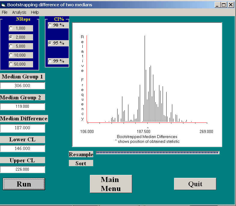
Notice that the distribution is not symmetric, with a rather scanty set of results on the left. This certainly is not quite what we would expect if these were means instead of medians. Notice that the obtained difference between the medians is 187, with confidence limits of 146 and 226. These limits are surprisingly symmetric about the obtained median difference (being 41 units below 187, and 39 units above 187). That does not always happen, though it did here. The limits were even symmetric when I looked at 90% or 99% intervals.

Because the confidence interval on the median difference does not include 0.0, we can safely conclude that the difference is significant.

A second example--a bad one

I have deliberately chosen an example that works poorly, just to illustrate the remarks I made at the top of this page. Werner, Stabenau, and Pollin (1970) asked mothers of normal and schizophrenic children to tell stories about ambiguous pictures. They scored for the number of stories, out of 10, that exhibited a positive parent-child relationship. They were hoping to show that parents of schizophrenic children were likely to tell stories with fewer positive relationships. (However, had they found what they were looking for, they still would not have been able to separate cause and effect.) The data are found in TAT.dat, where the first group is the parents of normal children.

The results of running this analysis are shown below.

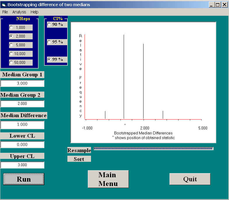
Here you can see that the medians of the two groups were 3 and 2, with a 95% confidence interval of 0.0 and 3.0. Because the interval includes 0.0, we can not reject the null hypothesis that the number of positive relationships in stories is the same in the two groups. (A t test, with means of 3.55 and 2.1 would reject the null, with t = 2.662, p = .011 (two-tailed). The confidence limits on the difference between means would be 0.347 and 2.55.) The results of using a randomization test (to be described later) to test differences between means can be seen at Randomization on TAT.