![]()
At one level the bootstrapping procedures for means are among the simplest. And a cursory reading of something like Simon & Bruce (2000) Resample Stats makes it appear completely straightforward. Actually it isn't all that straightforward, and as you read the literature you find that it can be more than a little confusing. In fact, it can be a real mess.
There are several different methods for bootstrapping a single parameter. I will work primarily with the mean because it is the simplest. In fact, in general our parametric procedures do quite nicely at producing confidence intervals on the mean, and we rarely need to look to things like bootstrapping. However, the fact that you can be counted on to know quite a bit about the mean makes it much more sensible to start there. Much of what is here carries over rather obviously to other measures.
The percentile method is the most straightforward. Suppose we have a sample
of 20 scores with a sample mean of 15. For the percentile method we simply draw
a large number of bootstrapped samples (e.g. 1000) with replacement from
a population made up of the sample data. We determine the mean of each sample,
call it![]() ,
and create the sampling distribution of the mean. We then take the
,
and create the sampling distribution of the mean. We then take the ![]() and
the 1-
and
the 1-![]() percentiles (e.g. the .025*1000 and .975*1000 = 25th and 975th bootstrapped
statistic), and these are the confidence limits.
percentiles (e.g. the .025*1000 and .975*1000 = 25th and 975th bootstrapped
statistic), and these are the confidence limits.
The percentile methods seems sensible, but actually it is a bit odd. The confidence limits are actually the limits on the sampling distribution of the mean, rather than some sort of limits on the parameter. In other words, if these limits should turn out to be 11 and 19, we are making a confidence statement on the probability that any future bootstrapped mean will lie between 11 and 19, whereas we want to be making a confidence statement on the value of mu(m).
If we are dealing with the sample mean, that isn't such a problem. We know the distribution of the mean to be symmetric for reasonable sample sizes, so things work out fine.
I give credit for this method to Clifford Lunneborg, though it is not original with him. The method is implicit in the writings of a number of people, but it stands out most clearly in Lunneborg's book: Data analysis by resampling.
Suppose for the sake of exposition that the sampling distribution of the mean obtained by bootstrapping came out to be highly skewed. (For means this would only happen in the extreme, but for other statistics it would be more common.) Assume that the bootstrapped distribution looks like the one that I have drawn (badly) below, where "a" represents the distance from the mean of the distribution (equal to the mean of the original sample) down to the 2.5th percentile, and "b" represents the distance up to the 97.5th percentile. I have deliberately drawn them so that a and b are not equal. I will represent the obtained value of the statistic in question by S, which is just my generic symbol for some statistic.
The true value for m could be way down to the left, and the obtained value would still be reasonable. In other words, m could be as low as (S - b), and the obtained statistic would still be a (barely) predictable outcome. But if m were up somewhere near the right tail, we would not expect to get a value as low as the one we obtained. In other words, m could not be any higher than (S + a) for the obtained to be likely. (By likely, I mean likely to occur 95% of the time or more.)
But this last paragraph means that the two confidence limits are (S - b) and
(S + a). In different notation, using the mean as the statistic, the confidence limits are (![]() -
(.975%tile -
-
(.975%tile - ![]() ))
and (
))
and (![]() +
(
+
(![]() -.025%tile)).
This looks just the opposite of what we said before, because the percentile
method gives (
-.025%tile)).
This looks just the opposite of what we said before, because the percentile
method gives (![]() -
a)
and (
-
a)
and (![]() + b),
whereas Lunneborg's method gives (
+ b),
whereas Lunneborg's method gives (![]() - b)
and (
- b)
and (![]() + a).
Things look backward, and logically Lunneborg is right. The reason why this
doesn't come up when we normally talk about confidence limits, is that with a
symmetric bootstrapped (or sampling) distribution, it doesn't make any
difference. In that situation a = b.
+ a).
Things look backward, and logically Lunneborg is right. The reason why this
doesn't come up when we normally talk about confidence limits, is that with a
symmetric bootstrapped (or sampling) distribution, it doesn't make any
difference. In that situation a = b.
Let's leave bootstrapping for a minute, and just concentrate on standard
confidence limits in parametric statistics. Again we will focus on the mean. We
know that the usual confidence limits can be found as ![]() .
We can solve for these limits just by taking the sample mean,
.
We can solve for these limits just by taking the sample mean, ![]() ,
finding the critical value of t from Student's tables (for reasonable
sample sizes it will be a bit more than 2.0), and multiplying by the standard error
of the mean, which is just the standard deviation of the sample divided by the
square root of n. Notice that these limits will be symmetric because +t
and -t will be equal except for the sign. This discussion will form the
basis for the next section on bootstrapped t intervals.
,
finding the critical value of t from Student's tables (for reasonable
sample sizes it will be a bit more than 2.0), and multiplying by the standard error
of the mean, which is just the standard deviation of the sample divided by the
square root of n. Notice that these limits will be symmetric because +t
and -t will be equal except for the sign. This discussion will form the
basis for the next section on bootstrapped t intervals.
The last type of confidence intervals that I will spend much time on are what Efron has called bootstrapped-t intervals. These are actually surprisingly like the traditional intervals, but with a twist. To calculate the traditional intervals, we had to use the tables of the Student t distribution. But Gosset originally derived that distribution on the assumption that we were sampling from a normal population. And the whole purpose behind bootstrapping is to get away from making that kind of assumption. But if we aren't going to assume normality, and therefore we turn up our noses at the (symmetric) Student t distribution, we have a problem.
Well, no we don't. Suppose that we took our original sample, treated it as a
pseudo-population, drew B bootstrapped samples, and calculated ![]() and s from on each. From these statistics we could solve for t*, where
the asterisk is used to indicate that each of these is a t calculated on a
bootstrapped sample. Now all we need are the 2.5% and 97.5% cutoffs of the t
distribution we would have without assuming normality. And we can get those
cutoffs just by drawing many bootstrapped samples, and calculating t* for
each sample (i.e. for each sample we calculate
and s from on each. From these statistics we could solve for t*, where
the asterisk is used to indicate that each of these is a t calculated on a
bootstrapped sample. Now all we need are the 2.5% and 97.5% cutoffs of the t
distribution we would have without assuming normality. And we can get those
cutoffs just by drawing many bootstrapped samples, and calculating t* for
each sample (i.e. for each sample we calculate ![]() ,
where
,
where ![]() is the mean of the ith
bootstrapped sample,
is the mean of the ith
bootstrapped sample, ![]() is the
mean from our original sample, and s* is its standard deviation.)
is the
mean from our original sample, and s* is its standard deviation.)
After drawing B bootstrapped samples, we take the resulting sampling
distribution of t* and find its 2.5% and 97.5% cutoffs, and substitute
those, instead of tabled values, in the traditional formula. This gives us![]() .
.
Notice that these limits are similar to Lunneborg's, in the sense that I have swapped the 2.5 and 97.5th percentiles from what we might normally expect. And I did it for the same reason that Lunneborg did.
This is the procedure implemented in the programs associated with this set of pages.
I don't want you to think that I have solved all the problems and given you the best estimates. Efron has spent 20 years on this problem and, along with a number of other people, he has come up with better limits. Unfortunately these limits are a bit unwieldy to calculate. But at least I should tell you what he has done.
The first solution is a correction for bias, and hinges on the fact that the sample estimate may be a biased estimate of the population parameter. Efron estimates this bias and removes it from the calculation of the interval.
The second problem that concerned Efron is that the standard error of the sampling distribution may change with different values of q, the parameter that we are trying to estimate. From what you have seen above, if the standard error depends on q, the width of the interval will vary with q. Efron attempted to compensate for this widening and narrowing. The solution that he came up with is called the BCA interval approach, standing for "bias correction and acceleration." The procedure is too complex to go into here, but is presented clearly in Efron and Tibshirani (1983).
I have presented the material here in the context of finding limits on the population mean. I did that because it is the easiest to talk about. But pretty much everything that I said here can be applied to other statistics, although calculating some of them may be difficult. For example, we know that the standard error of the mean is the standard deviation of the sample divided by the square root of n. It is easy to make that calculation, and substitute the standard error into our formula. But what is the standard error of the median if the distribution isn't normal? That's a difficult one. We may have to estimate it by drawing bootstrapped samples within bootstrapped samples. That isn't fun, and that is why you won't see a good bootstrapped median procedure in version 1.0 of my program. I will get around to it later, in which case you will want to download the latest version from the web site.
Caitlin Macauley (1999, personal communication) collected mental status scores on 123 people between the ages of 60 and 95. One of her dependent variables was a memory score on the Neurobehavioral Cognitive Status Examination. As you might expect, these data were negatively skewed, because some, but certainly not all, of her participants had lost some cognitive functioning. In fact the distribution was extremely skewed, as seen below.
Macauley was particularly interested in forming a confidence interval on the median, but we will use this example to form a 95% confidence limit on the mean. This is an interesting exercise because it illustrates just how robust the central limit theorem is.
The figure below shows the results of using Resampling.exe to generate 95% confidence limits on the mean. These limits are 8.65 and 9.60, and are remarkably symmetric about the mean. The lower limit is 0.489 units below the mean, while the upper is 0.465 units above the mean. We can also see that the distribution of means is approximately normal, and the standard error of this bootstrapped distribution (its standard deviation) is 0.241.
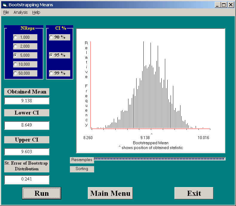
If we had ignored the fact that the original distribution is very negatively skewed, and just calculated confidence limits assuming that n was sufficiently large for the sampling distribution to be normal, we would have a standard error of 0.247 and 95% confidence limits of 8.65 and 9.63. Notice how close the normal approximation comes even though we know that the distribution is markedly skewed. Of course we are talking about a sample of 123 observations, and it is the large sample size that saves us.
The general conclusion of people working in this field is that there really is no great advantage to using bootstrapping to set confidence limits on a mean. The reason for covering it here is that it is the simplest way to begin, and, in fact, our results agree very well with theory. We will see that this will not always be true when it comes to estimating different parameters.
![]()
![]()
Last revised: 06/25/02