![]()
I have spent an inordinate amount of time on the problem of bootstrapping correlations, and have come back to the simplest solution. You might expect that bootstrapping a correlation coefficient is a "no-brainer," but it is not. The literature seems extremely clear, until you get down to the nitty-gritty of implementation. Then it is not so clear.
I would suggest that one of the best places to see the importance of a confidence interval is in the area of correlation. I can easily image situations where I would be particularly interested in whether a mean, or a difference between two means, is significantly different from 0.0. But it is harder to imagine situations in which I would get all excited by being told that a correlation is significantly different from 0.0. My response might actually be: "We'll so what; how large is it?" For example, I am sure that there is probably a correlation between SAT scores and subsequent success in life (however we might want to measure that). But if that correlation is only .20, accounting for 4% of the variation, that is a fact that I could happily live without knowing. However, if it is .50, that's a big deal. So, I would be particularly eager to see some sort of confidence limits on that correlation.
Incidentally, if we have confidence limits, we also have a test of the standard null hypothesis. If those limits include 0.0, the correlation is not significant.
The simplest way to generate confidence limits on a correlation coefficient is to use the method that I referred to as the "percentile method" when talking about confidence limits on the mean. In this approach, we simply draw a large number of bootstrapped samples, or size n, with replacement, from a population consisting of the original data. We draw samples pairwise, meaning that when we sample an X value from personi or objecti, we also draw the corresponding value of Y. For each bootstrapped sample we calculate rj*, j = 1 to B, where B is the number of bootstrapped samples.
For the 95% confidence limits, for example, we then sort the resulting distribution of rj*, and take the values falling at the 2.5 and 97.5 percentiles of rj* as our confidence limits. Thus, if we set B = 1000, when the rj* are sorted, the confidence limits will be the 25th and 975th values.
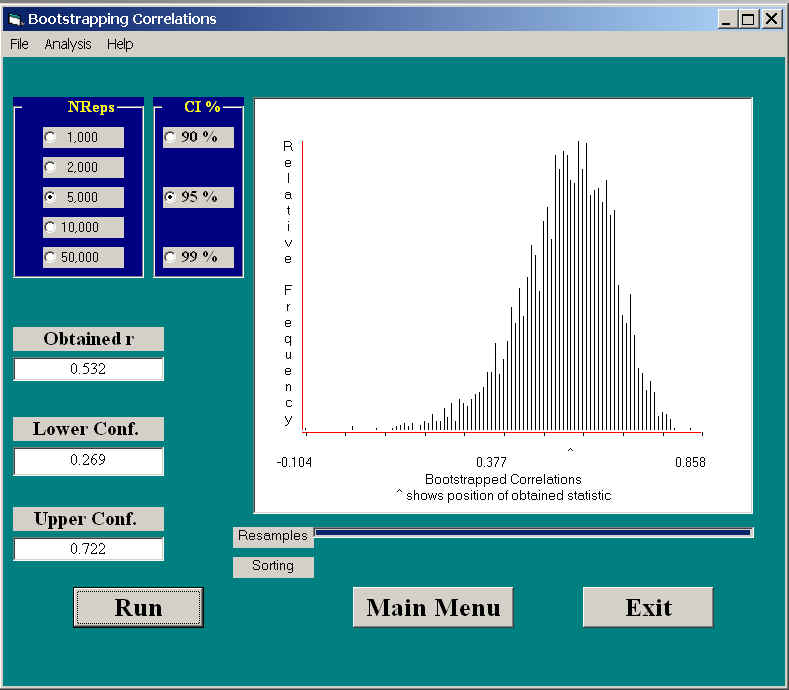
Elsewhere I have described a study by Katz, Lautenschlager, Blackburn, and Harris (1990). In this study they asked one group of participants to answer a set of SAT-like questions without first having read the passage on which those questions were based. They found that the participants in their study could perform at significantly greater than chance levels, presumably due to various test-taking skills, such as eliminating unreasonable-sounding answers. Katz et al were interested in knowing how well students' performance on this test could be predicted from their performance when they took the SAT for college admission. They collected SAT scores for these students, and correlated those scores with their performance on Katz et al's task. This correlation, for n = 28, was .532, which was significant by a standard t test.
The following figure shows the results of drawing 5000 bootstrapped samples, each of n = 28, with replacement from the original data set. As you can see, the sampling distribution of r is negatively skewed, as we would expect. The 95% CI are given as .269 and .722. Those are fairly wide intervals, but n = 28, which is not very large for setting confidence limits. In addition, confidence limits have an unpleasant habit of generally being larger than we would like. Notice that the limits do not include 0.0, which confirms that the correlation is significant, using a test that does not rely on bivariate normality of the data.
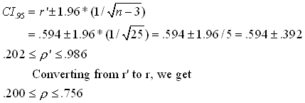
By the nature of the variables used in this study, it is reasonable to expect that an assumption of bivariate normality is not terribly unreasonable. That means that we could have formed confidence limits using Fisher's transformation, computed as r' = 0.5*ln[(1+r)/(1-r)]. This transformation produces a nearly normal sampling distribution with a mean of r' and a standard deviation of 1/sqrt(n-3). This leads to the following 95% confidence limits:
Notice that these limits are somewhat wider than those obtained by bootstrapping. especially at the lower end. This is in line with results that others, see especially Rasmussen (1987), have found, and that prompted Efron to search for better limits. (References are given below.)
You might think that I have just passed up an obvious solution to the problem. Why don't I convert everything to r', bootstrap r', set confidence limits on r', and then convert everything back to r. That seems like a simple solution, and, because r' is normally distributed with a known standard error, everything out to work out. Yeah, I thought so too for a few minutes. Well, first of all, that transformation depends on an assumption of bivariate normality. Second, it wouldn't make any difference. Notice that the transformation for r to r' is a simple monotonic transformation. In other words, we just stretch the scale a bit--more at one end than the other. But that means that the 25th value of r' in a sorted array will translate directly back to what would have been the 25th value of r if we sorted that array. So we go to a lot of work, and end up in exactly the same place.
Efron (1988) has remarked on this issue. He noted that if there is some sort of transformation that will normalize a set of data, and if it is a monotonic transformation, then it won't matter whether we use the transformed or untransformed data. But that means that the standard percentile approach to setting confidence limits is "transformation invariant." To quote Efron, "The bootstrap percentile methods, including various corrections, are transformation invariant. This means that the methods can be applied on the original scale, (or) the (transformed) scale, with the assurance that if any normalizing transformation exists, then that transformation will in effect be automatically incorporated into the computation of the bootstrap confidence intervals." We don't even have to know how to carry out such a transformation, or what it would look like, just so long as one exists. That's neat!
You might think, as I did, that what I referred to as Lunneborg's approach, when discussing confidence limits on the mean, would be a nice alternative. You should recall that we took the distance from the sample mean to the 97.5th percentile, and subtracted that from the mean to get the lower bound. We then took the distance from the 2.5th percentile to the mean, and added that to the mean to get the upper bound. It looked backward, but it made sense. So why not do that here?
Why not, indeed. But think back to the paragraph in which I stated that the percentile method is transformation invariant. When we have a symmetric distribution, it won't matter whether we use Lunneborg's method or not, because the two distances will be equal. But if we get the same answer when we use r or r', and if r' is a symmetric sampling distribution, then why should we get different answers whether we use the standard percentile method or Lunneborg's method? But of course we will. That is my problem. If nothing else, that simply points to the fact that if you are looking for what I say to answer all your questions, you're going to be disappointed. I'm confused too.
My reading of the literature on confidence limits on correlation coefficients is not particularly comforting. Efron and others have sought for ways to improve the solution, and those approaches seem to work in some cases, but not always. I am left with the feeling that Fisher's transformation works "well enough," and seems to err of the conservative side. I could not, however, put together this set of pages on bootstrapping without discussing the correlation coefficient.
Efron, B. (1988). Bootstrap confidence intervals: Good or bad? Psychological Bulletin, 104, 293-296.
Efron, B. & Tibshirani, R. (1986). Boostrap methods for standard errors, confidence intervals, and other measures of statistical accuracy. Statistical Science, 1, 54-77.
Lunneborg, C. E. (1985). Estimating the correlation coefficient: The bootstrap approach. Psychological Bulletin, 98, 209-215.
Rasmussen, J. L. (1987). Estimating the correlation coefficient: Bootstrap and parametric approaches. Psychological Bulletin, 101, 136-139
Strube, M. J. (1988). Bootstrap Type I error rates for the correlation coefficient: An examination of alternative procedures. Psychological Bulletin, 104, 290-292.
![]()
![]()
Last revised: 09/20/2004