Multiple Comparisons with
Repeated Measures

David C. Howell

One of the commonly asked questions on listservs dealing with statistical issue is "How do I use SPSS (or whatever software is at hand) to run multiple comparisons among a set of repeated measures?" This page is a (longwinded) attempt to address that question. I will restrict myself to the case of one repeated measure (with or without a between subjects variable), but the generalization to more complex cases should be apparent.

There are a number of reasons why standard software is not set up to run these comparisons easily. I suspect that the major reason is that unrestrained use of such procedures is generally unwise. Most people know that there are important assumptions behind repeated measures analysis of variance, most importantly the assumption of sphericity. Most people also know that there are procedures, such as the Greenhouse and Geisser and the Huynh and Feldt corrections, that allow us to deal with violations of sphericity. However many people do not know that those correction approaches become problematic when we deal with multiple comparisons, especially if we use an overall error term. The problem is that a correction factor computed on the full set of data does not apply well to tests based on only part of the data, so although the overall analysis might be protected, the multiple comparisons are not.

A Comment on Multiple Comparison Procedures

I need to start by going over a couple of things that you may already know, but that are needed as a context for what follows.

Error Rates

Statisticians mainly worry about two kinds of error rates in making multiple comparisons.

• Per Comparison Error Rate
  • This is the probability that any one contrast will be found significant by chance. In other words, it is the probability of making a Type I error on that contrast. Of course, you can't make a Type I error unless the underlying null hypothesis is true. Normally we represent the per comparison error rate by α.
• Familywise Error Rate
  • This is the probability that we will make at least one Type I error in a set (family) of comparisons. If we compare Treatment1 against Treatment2, Treatment 3 against Treatment4, and Treatment1 against Treatment4, the familywise error rate is the probability that our set of three conclusions will contain at least one Type I error. In the example I just gave, where the contrasts are independent, the familywise error rate would be approximately 3*α = 3*.05 = .15. (If the contrasts are not independent, .15 would represent a maximum.

In general (but see below) a priori tests are often run with a per comparison error rate in mind, while post hoc tests are often based on a familywise error rate.

Calculations

Forget about all the neat formulae that you find in a text on statistical methods, mine included. Virtually all the multiple comparison procedures can be computed using the lowly t test; either a t test for independent means, or a t test for related means, whichever is appropriate.

Certainly textbooks give different procedures for different tests, but the basic underlying structure is the t test. The test statistic itself is not the issue. What is important is the way that we evaluate that test statistic. So I could do a standard contrast, a Bonferroni test, a Tukey test, and a Scheffé with the same t test, and I'd get the same resulting value of t. The difference would be in the critical value required for significance.

This is a very very important point, because it frees us from the need to think about how to apply different formulae to the means if we want different tests. It will allow us, for example, to run a Tukey test on repeated measures without any new computational effort—should that be desirable.

A Priori and Post Hoc tests

• A priori tests
• In theory, a priori tests are tests that have been planned before the data were collected, and are not based on any information about the resulting sample means. (Forgive me for not italicizing the Latin, but editors have finally beat that out of me.) What I think is important is that a priori tests are a small set of planned comparisons.
• Because with a priori contrasts we are not usually running many contrasts, tradition ignores, I believe unwisely, the effect on the familywise error rate, and allows each test to go forward at alpha = .05—the per comparison error rate. I don't believe that I have seen a text that recommends other than to run each of those at the .05 level, though I really doubt the wisdom of doing so.

 

• Post hoc tests
  • In theory post hoc tests are tests that were decided upon after the data have been collected. Generally the researcher looks at the set of means, notices that two means are quite different, and says to herself "I wonder if those means are significantly different." 
  • You might suspect that post hoc tests would normally be few in number, because there may be only a few means that are very different from one another. However, we always treat post hoc contrasts as if we are comparing all means with all other means. The reasoning is that this is just what you did. You saw two means that were very close, and lost interest in them. Then you saw two means that were moderately different, and debated about testing them. Then you saw two means that were quite different, and pounced on them to be tested. In essence, your brain has looked at all pairwise differences and picked on the few largest ones. All we are doing is to "credit" you with mentally having made all pairwise contrasts in your head, even though you just did the biggest ones on paper.
  • What virtually all post hoc procedures do is to assume that you are actually running, in your head if not on paper, all k(k- 1)/2 pairwise contrasts, where k is the number of means in the set. The tests then adjust the critical value of the test statistic accordingly, thereby keeping the familywise error rate at, or near, .05.

Comparisons and Contrasts

Throughout this document I use the words Comparison and Contrast interchangeably. For what we are doing, they mean the same thing. I thought that I ought to spell that out to avoid confusion. 

Two Means versus Two Sets of Means

Again, I just want to spell out something that most people may already know. I will generally speak as if we are comparing Mean1 with Mean2, for example. However, the arithmetic is no different is we compare (Mean1 + Mean2 + Mean3)/3 with (Mean4 + Mean5)/2. In other words, we can compare means of means. If you had two control groups and three treatment groups, that particular contrast might make a lot of sense. Again, the arithmetic is the same once you get the means.

The Nature of the Repeated Measure

It is very important to make a distinction between repeated measures, such as Time, Trials, or Drug Dose, where the levels of the variable increase in an orderly way, and repeated measures such as Drug Type, Odor, or Treatment, where the levels of the variable are not ordered. Although the overall repeated measures analysis of variance will be exactly the same for these different situations, the multiple comparison procedures we use will be quite different.

When we have a variable that increases in an orderly fashion, such as time, what is most important is the pattern of the means. We are much more likely to want to be able to make statements of the form "The effect of this drug increases linearly with dose, " or "This drug is more effective as we increase the dosage up to some point, and then higher doses are either no more effective, or even less effective." We are less likely to want to be so specific as to say "The 1 cc dose is less effective that the 2 cc dose, and the 2 cc dose is less effective than the 3 cc dose."

I am going to begin with the case where the repeated measure increases on an ordered scale. (I will avoid the issue of whether that scale is ordinal or interval.)

Repeated Measures with Ordinal Levels

The most common form of a repeated measures design occurs when participants are measured over several times or trials, and the Trial variable is thus an ordered variable. I will take as my example an actual study of changes in children's stress levels as a result of the creation of a new airport. This is a study by Evans, Bullinger, and Hygge (1998). I have created data that have the same means and variances as their data, although I have added an additional trial. (I made a guess at the pattern of covariances, and the results are the same as those that they reported.)

This study arose because the city of Munich was building a new airport. The authors were able to test children 1) before the airport was built, 2) 6 months after it was opened, 3) 18 months after it was opened, and, for my purposes, 4) 36 months after it was opened. They used the same children at each of the four times, and they had a control group of children in the same city but living outside the noise impact zone. (I have coded the Locations as 1 = Near Airport; 2 = Away from Airport.) The dependent variable I have chosen is epinephrine level in these children, which is a variable that is a known marker for stress. The measures at each interval have been labeled Epineph1, ..., Epineph4, but they could have equally well been labeled Time1, ..., Time4 .

The data are available at Airport.sav. (Internet Explorer will recognize this as an SPSS system file and download it. Other browsers may not. The raw data can be downloaded at Airport.dat.)

The descriptive statistics and the overall analysis of variance are shown below.

Descriptives

LOCATION = 1 (Near)

LOCATION = 2 (Away)

A glance at the means will reveal that those who live close to the new airport show an increase in epinephrine levels (and thus presumably stress) over time, while those who live away from the airport remain relatively stable. Mauchly's test is shown next. Although it is of borderline significance, the Greenhouse - Geisser, and Huynh - Feldt corrections differ trivially from 1.00. I probably would not worry about violations of the symmetry assumption. However I am concerned that the variances of the Near condition are appreciably larger than the variances of the Away condition. (This test is shown as Levene's Test below.) Because of this, I think that it is very important to be careful how we set up any subsequent analyses. We want to use error terms that are appropriate to the means being compared. (Don't use an error term from the overall analysis when examining simple effects for the Near condition, etc.)

The following analysis of variance shows that all of our effects are clearly significant, whether we correct for sphericity or not. We can have confidence about those results, but we still want to be cautious in subsequent analyses.

If these were my data, I would probably stop right there with a graphical display of the effects. (I am of the "minimalist" school. I would, however, calculate some measure of effect size, but I will not take that digression here.) However, most people would want to push ahead and tie down the effects more closely. There are two things that we could do with the Time variable. One possibility, which strikes me as not useful, would be to collapse over groups and look at the significant differences due to the main effect of time. But our eyes can see what the interaction supports, and that is that there is essentially no interesting Time effect for the "away" group, but there is one for the "near" group. It seems to me that the average of an effect and a non-effect is meaningless, and I see no point in pursuing that approach.

A better approach would be to take the significant interaction into account and look at the simple effects of Time at each level of location. For brevity, I will restrict myself to an examination of Time for the "Near" condition.

Tests on Within Subject Effects—Trend analysis

A polynomial function is just a function of the form  = aX² + bX + c. When "a" is 0, this is just the equation of a straight line. When "a" is nonzero, but "b" is 0, this is a quadratic (rising and then falling, or vice versa.) When neither "a" and "b" are 0, then we have a curve that generally rises, but starts falling off slowly at higher values of X. (See below.)

The idea behind a trend analysis is that we want to explore whether a polynomial function, linear or otherwise, will fit the data reasonably well. To put this slightly differently, we want to know whether there is a linear, quadratic, cubic, etc. relationship between Time and stress. To do this we will ask if a straight line fits the Time means. Then we will ask if a quadratic (a line that goes up and then down, or vice versa) is a reasonable fit to those means. We will set up our tests such that a significant effect means that the associated line fits the means at better than chance levels. [For further discussion of polynomial contrasts and their meaning, see Howell, 2002.

This question is easily addressed in SPSS and other software. For our example I am only going to apply it to the simple effect of Time at Near. Moreover, I am not going to use any of the "Away" data in computing the error term. I do this because I am sufficiently nervous about the differences in variability, and perhaps problems with sphericity, that I want my error term to be based only on the data that were collected under the Near condition. Then any differences in variance between the Near and Far conditions don't play a role in the analysis.

The way that I rule out the influence of the Away data is to ignore them completely. I instruct SPSS to restrict the analysis to the Near data.

The following graphics illustrate the pattern in the means after I used the Data/Select Cases command to restricted the analysis to only those cases where Location = 1.

Here we can see that there is a general increase from left to right, but that it levels off between times 3 and 4. This would suggest that we might have both a significant linear and a significant quadratic component. 

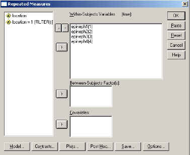
To run the analysis we first set up a standard repeated measures analysis, as shown in the dialogue box below, and then click on the "contrast" button. This will display the second dialogue box below. If that box does not show that you are requesting a polynomial test on Time, use the Change Contrast portion to make that selection. Then press Continue. (If you are changing to Polynomial, be sure to click on "Change" after you select the contrast!!)

The results are shown below, omitting what has already been shown in the original printout.

Here you see that we have both significant linear and quadratic components, but that the cubic component is not significant. Thus we can conclude that stress does increase linearly over time for children living near an airport, but that there is also a quadratic component reflecting the fact that the increase levels off, and even falls, at the last measurement. Those seem like reasonable results, and the trend analysis really answers the major questions that we would be interested in.

Tests on Between Subject Effects

I should point out in passing that we could easily make post hoc tests on the Between Subjects factor if we had more than two groups. (With two groups it would simply boil down to a t test between groups at each Time.) To do the post hoc analyses you would click the Post Hoc button in the dialog box above, and then select your favorite test. We could either do this with the full 2 × 4 design, or we could do separate analyses for each level of the repeated measure. I might use such an analysis to examine whether the groups started off the same at baseline (i.e. 6 months before the airport was opened). I suppose that I could also do this at one or more of the later times, but our interaction and plots already show us that the groups are diverging, and it is probably not critical at what time the study has sufficient power to first show us a difference between groups.

Remember, if you run multiple comparisons, such as the Tukey, between groups at each time, each set of comparisons is protected against an increase in the risk of Type I errors by the nature of the test. However, there is no protection from one time period to another. If you test between groups at times 1, 2, 3, and 4, the familywise probability of a Type I error is .05 at each period, but approaches .20 for the full set of comparisons. That is one reason why I strongly urge people to limit the number of tests they run, no matter what the nature of those tests.

This analysis has treated the levels of Time as if they are equally spaced. This is probably close enough for our purposes. I know of no way that you can set the metric in SPSS for a repeated measure, though you can specify a metric, via syntax, for a between-subjects design. (SPSS One-Way will allow you to specify contrast coefficients for between subject factors.)

Repeated Measures with Non-ordinal Levels of the Repeated Measure

Trend analysis is an excellent way to make sense of a repeated measure that increases in an ordered way, because it is the orderliness of the change that you care about. But many of our designs use a repeated measures variable than is not ordinal. 

I hate to use contrived examples, but I don't have anything at hand that would work nicely for an example. So what I will do is to modify the previous study by Evans, Bullinger, and Hygge. In fact, Hygge, Evans, and Bullinger published a study in 2002 that was based on this same basic piece of research, and they took 4 measurements on each child; namely Reading, Memory, Attention, and Speech perception. (They also measured at multiple times, but I'll ignore that.) I am going to take the data that I used in the earlier example, but rename the variables from Time1, Time2, Time3, and Time4 to Reading, Memory, Attention, and Speech. We will assume that these measurements represent a percentage change (with the decimal dropped) from Before Airport to After Airport, so that it makes sense to ask if reading scores changed more than memory scores, etc. Greater change represents greater deterioration.

The data can be found in a file named airport2.sav, where I have simply renamed the levels of the repeated measure. (Well, that's not quite honest. I changed the values a bit to make for more interesting results. Since the whole revised experiment is fictitious, I might as well go all the way and get data that I like.)

There is no point in reproducing the analysis of variance, because it will be essentially the same as the one you saw before. There will be a significant effect due to Location, Test, and Location X Test. The plot illustrates the results.

In this case, unlike the first example, it does make sense to wonder about differences between the individual means on each test. We might reasonably ask if attention was affected more by noise than was memory. (Unfortunately, this is not my field, and I can't come up with a basic theory that would make predictions here, but we can assume that if this were your study you would know enough about what you are doing to make those predictions.)

The first question that someone is likely ask is "How do I run a Tukey test on these means?" That is not a bad question, but I don't know a simple answer. But don't get discouraged, I know some other stuff that will be useful to you, and we will come up with a Tukey test if you really have to have one.

You need to remember that I started out by saying that there is nothing particularly mysterious about multiple comparison tests. Most of them, including the Tukey, boil down to running a bunch of t tests and then adjusting the significance level to take the appropriate control of Type I errors. For example, The Bonferroni test uses a straight-forward t test but then evaluates that t at α = .05/c, where c is the number of comparisons. The Dunn-Sidak test does the same thing, but with a slightly different adjustment to the critical value. So, if I wanted to compare Reading with Memory, Memory with Speech, and Attention with Speech using a Bonferroni correction, it would be perfectly appropriate and correct for me to run a paired t test between Reading and Memory means, then the Memory and Speech means, and finally the Attention and Speech means. I have now run c = 3 tests, so I would reject the null hypothesis in each case if the associated p value were less than .05/3 = .0167. It is important to emphasize that you either pick a select set of comparisons on the basis of theory, in which case your correction is not particularly severe, or you run the full set of all pairwise differences, in which case your correction is likely to be quite severe if you have many levels of the repeated measure. You will probably recognize that the first alternative is a set of a priori comparisons, while the second is post hoc.

To illustrate what I am doing, I will first lay out the comparisons that I presumably came up with on the basis of theory. The results are below

I said earlier that the traditional coverage of a priori tests in most texts assumes that you are not going to make any correction for familywise error rate. (That term is usually brought in when we get to post hoc tests.) I don't think that is a good strategy. I would like to see all contrasts protected so as to restrict familywise error rates to p = .05, or at least p = .10. 

Taking the traditional, and I think too liberal, approach, we would conclude that there are significant differences for all three of these contrasts. 

I would prefer a different approach. I want to specify my contrasts in advance (i.e. a prior), which gives me fewer than all possible contrasts. But at the same time, I want to control the familywise error rate, perhaps with a Bonferroni test. If I use the Bonferroni, I will have 3 comparisons, with a familywise error rate of .05, and thus run each test at the .05/3 = .0167 level. Using this approach, the difference between Reading and Memory would be significant, but the rest of the differences would not be.

But suppose that you have a co-investigator, or an editor, who insists on the more traditional post hoc tests. All this really means, as far as the Bonferroni post hoc test is concerned, is that you do exactly the same thing, except for all pairwise contrasts, and correct using c = k(k-1)/2, where k = the number of means. I have shown that result below, of which the earlier result is a subset.

We have four means, so c = k(k-1)/2=4(3)/2 = 6, and thus we will require a probability of .05/6 = .008 for significance. This means that Reading is significantly different from all other tests, but the other tests are not different from each other.

A Different Way to do the Same Thing

I have run each of these comparisons using simple t tests, and I can do that from beginning to end in about 30 seconds. But perhaps you want a more formal way to do it, or one that appears to have the blessing of SPSS. David Nichols, at SPSS, put together a set of SPSS macros that you can use for this purpose. They can be found at RMPOSTB.SPS or RMPOSTB2.SPS . All you have to do is to go to that site and click on the link to post hoc tests for repeated measures. Then download rmpostb.sps to the same directory that you have you data in. Then write the following syntax file

include rmpostb.sps.
rmpost var=Reading memory attentin speech /alpha = .05.
Execute.

The result is shown below.

If you divide the Mean Difference by the Standard Error of the Difference, you will get exactly the t values  that I obtained. And if you look at his pattern of significance, you will see that it is exactly the same as mine— because he calculated significance exactly the way that I did.

So why did I go through all that I did if I could point you to a macro that David Nichols wrote? Well, first of all, I am a professor (well, a retired one, but we never give up), and professors want to teach people things. Second, I think that it is far easier to run all those nice simple t tests than to download a macro and figure out how to run it. Third, and more importantly, my approach will let you do what you have secretly wanted to do all along- -run a Tukey test on the means. (It would be difficult to modify Nichol's macro to do that.)

An Even Easier Way

I was not aware of it, but you can actually use SPSS to get these comparisons if you want all pairwise ones. (If you don't want all pairwise contrasts, just promise yourself that you will only look at the important ones and ignore the others.) Shanti Ganesh at the Behavioural Science Institute of Radboud University in the Netherlands sent me a message pointing out a more direct solution. His message said, in part,

Now why didn't I know that?

Tukey—Finally

I know that most people are really looking for a way to run Tukey's test, because that is what they have been told is the best post hoc test around. (We could quibble over what really is the best test, and if you want to give that title to John Tukey, I won't argue too much, though I prefer another test. He was a brilliant man and made many worthy contributions to statistics.) So how do you do Tukey's test with the resources at hand?

If you go to a good statistical methods text, and I might as well recommend my own, you will find that tests such as Tukey's are based on what is known as the Studentized Range Statistic. I discuss the Studentized Range Statistic in my book, and point out that the critical value of the test statistic is dependent on the number of means in an ordered series. What this means for Tukey is that the constant we will use, commonly called r for "range," will be equal to the number of means we are examining. For our example, we are making comparisons among 4 means, so r = 4.

I also point out that the Studentized Range Statistic (q) is directly tied to the t statistic. Specifically, q = t√2. This means that we could convert a t test on the means to a q statistic, just by multiplying t by the square root of 2. Alternatively, we could look up the critical value of q required for Tukey's test, and convert that to a critical value of t by t = q/√2. That's easy enough. You don't even need to open up a book, because you can find a table of the Studentized Range Statistic on the web at http://cse.niaes.affrc.go.jp/miwa/probcalc/s- range/srng_tbl.html. The author of that table used k instead of r. Just be aware that the first table on that page is for alpha = .10, so scroll down to the alpha = .05 table.

For our example we have the 4 means for the Near condition, therefore r = 4, and we have 99 df for error. (Remember, I have restricted myself to the Location = Near condition, and I am running separate t tests for each pair.) Going to the table of the Studentized range we have q_crit = 3.71 (with interpolation). We can convert this to a critical value of t by t = q/√2 =3.71/√2 = 2.62. This means that all we have to do is run all pairwise t tests among the means of the repeated measure, and reject the null hypothesis when the computed value of t is greater than 2.62. For our example this would mean that we would conclude that Reading is different from all other tasks, but the other tasks do not differ among themselves. And, because of the way the fact that we have used a Tukey test, the familywise error rate is .05.

Why am I not Satisfied?

I have just written an answer to a questions that dozen and dozens of people have asked me over the years, but I am not as satisfied as I imagine those people will be. Why? The reason is that I am not happy with any of the traditional multiple comparison procedures. It isn't that I don't respect them, or that I think that they are incorrect. It is that I fear that they make it too easy to take the easy way out, and, in so doing, are too conservative.

If you truly need to compare every mean with every other mean, and you actually care about all of those k(k-1)/2 comparisons, then tests like the Tukey are for you. But you pay a pretty stiff price with a conservative test. When you guard against all sorts of chances of making an error, you need to put up a pretty good barrier.

I would much prefer to see people limit their questions to a relatively few comparisons, and thus pay a lower price to control the familywise error rate. If there are a bunch of tests where you really don't care what the answer is—either because it is almost certain to be significant or nonsignificant, or because it is a meaningless question, then don't run that comparison. If you can cut down the comparison's you really care about, you may find that the critical value for the resulting few Bonferroni tests is less than the critical value for something like the Tukey. In that case, go with the Bonferroni (or the Dunn-Sidak, which is slightly more powerful). It is perfectly acceptable to calculate the size of the critical value under a number of different tests, and then choose the test with the smallest critical value. 

Why Didn't I Talk about the Other Contrast Options in SPSS?

When I talked about how to tell SPSS that you wanted to run a polynomial trend analysis, I showed you a dialog box (opened by the Contrast button) that contained other contrasts. These were contrasts such as Simple, Deviation, etc. These contrasts are preset to do things like compare each group with the last group, or compare each group with the one before it, or compare each group with the mean of the others, etc. There is nothing wrong with these contrasts, but I have never found them particularly useful, and didn't see any particular reason to single them out for coverage. (Besides, I never remember which one does what, and have to look them up each time I want them, or run them and examine the results to find out what they did.) If they answer the questions you want to ask, them by all means use them. Otherwise find some other way.

Finally

You may have noticed that I have been running individual t tests, based purely on the data in the relevant groups. For example, when I compared Reading to Memory, I only used those two sets of data. David Nichols does the same thing in his macro. 

The traditional approach is to grab the error term (MS_error) from the overall anova and use that in your t tests. I am not recommending that approach here because it is too sensitive to violations of assumptions—particularly the assumption of sphericity. If you can convince yourself that this is OK, then go back and recalculate your results by hand, substituting MS_error . But in general, you are better off following two simple guidelines: 

1. Run as few contrasts as possible.
2. Use only the data involved in those contrasts to run the contrasts.

That's all folks!

But if you have any questions or corrections, you can write me at mailto:David.Howell@uvm.edu. If you have a better example than mine, or one that illustrates other issues, I would love to have the data. In fact, for a really good example I might trade the analysis for a chance to use the data in an example.

Evans, G.W., Bullinger, M., & Hygge, S. (1998) Chronic noise exposure and physiological response: A prospective study of children living under environmental stress. Psychological Science, 9, 75-77.

Howell, D. C. (2002) Statistical Methods for Psychology, 5th ed.. Belmont, CA: Duxbury Press.

Hygge, S., Evans, G.W., & Bullinger, M. (2002) A prospective study of some effects of aircraft noise on cognitive performance in schoolchildren. Psychological Science, 13, 469-474.

  My HomePage]

Created: 11/02/2002