

When we look at the bootstrap approach to correlation, we will see a procedure in which a very large number of resamples were drawn pairwise from a pseudo-population consisting of the observations in the original sample. The data consisted of pairs of observations on each experimental unit. Units are drawn, with replacement, from the pseudo-population, and a correlation coefficient is computed. After this procedure has been repeated B > 1000 times, the resulting correlation coefficients form the sampling distribution of r. We will then be able to set confidence limits on r using this sampling distribution. As I said earlier, bootstrapping focuses primarily on parameter estimation, whereas randomization tests focus primarily on hypothesis testing.
When we apply randomization tests to bivariate data, our primarily goal is different. We want to test a null hypothesis, usually that r = 0. We do this by holding one variable (e.g. X) constant, and permuting the other variable (Y) against it. Because each Xi is randomly paired with a value of Y, the expected value of the correlation is 0. By repeating this process a large number of times, we can build up the sampling distribution of r for that situation in which the true value of r is 0.0. We can either create confidence limits on ρ (a strange undertaking in this case), or we can increment a counter to record the number of times a correlation coefficient from a bivariate population where r = 0.0 exceed the obtained sample correlation (for either a one- or a two-tailed test.)
Elsewhere I have discussed a study by Katz et al. (1990) that dealt with asking students to answer SAT-type questions without having read the passage on which those questions were based. (For non-U.S. students, the SAT is a standardized exam commonly used in university admissions.) The authors looked to see how performance on such items correlated with the SAT scores those students had when they applied to college. It was expected that those students who had the skill to isolate and reject unreasonable answers, even when they couldn't know the correct answer, would also be students who would have done well on the SAT taken sometime before they came to college.
The data for that study follow. The data have been created to have the same correlation and descriptive statistics as the data that Katz et al. collected.
Score   58  48  48  41  34  43  38  53  41  60  55  44  43  49
SAT    590 590 580 490 550 580 550 700 560 690 800 600 650 580
Score   47  33  47  40  46  53  40  45  39  47  50  53  46  53
SAT    660 590 600 540 610 580 620 600 560 560 570 630 510 620
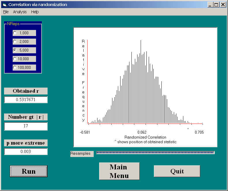
The randomization test is shown below.
In this figure you can see that the correlation obtained by Katz et al. (1990) on the original data was .532. You can also see that the sampling distribution of r under randomization is symmetrical around 0.0, and that 17 of the 5000 randomizations exceeded +.532. This gives us a probability under the null of .003, which will certainly allow us to reject the null hypothesis. This is a two-tailed test, and, because the distribution is symmetric for r = 0, you will not go far wrong if you cut the probability in half for a one-tailed test.
This is a good place to again make a point that was made earlier about the difference between bootstrapping and randomization procedures. I make it here because the difference between the two approaches to correlation is so clear. (This section was written in an earlier version where I discussed bootstrapping before randomization. It should be possible to follow this even though we have not yet discussed bootstrapping in any detail.)
When we bootstrap for correlations, we keep Xi and Yi pairs together, and randomly sample pairs of scores with replacement. That means that if one pair is 45 and 360, we will always have 45 and 360 occur together, often more than once, or neither of them will occur. What this means is that the expectation of the correlation between X and Y for any resampling will be the correlation in the original data.
When we use a randomization approach, we permute the Y values, while holding the X values constant. For example, if the original data were
45 53 73 80
22 30 29 38
then three of our resamples might be
|
45 53 73 80 |
45 53 73 80 |
45 53 73 80 |
Notice how the top row always stays in the same order, while the bottom row is permuted randomly. This means that the expected value of the correlation between X and Y will be 0.00, not the correlation in the original sample.
This helps to explain why bootstrapping focuses on confidence limits around ρ, whereas the randomization procedure focuses on confidence limits around 0.00 (or counts the number of bootstrapped correlations more extreme than r). I see no way that you could apply a permutation procedure with the intent of having the results have an expectation of ρ. Similarly, I don't see how you would set up the bootstrap to be centered on 0.00 (unless you bootstrapped (r* - r), which is an interesting possibility, and one that I will think about).
We can accomplish the same thing using R. We simply creqte our X and Y values, permute X, and compute the percentage of times that the resampled data produce a value of r greater than the obtained value of r. The code is below.
# A test on a correlation coefficient.
# A test on a correlation coefficient.
Score <- c(58, 48, 48, 41, 34, 43, 38, 53, 41, 60, 55, 44, 43, 49, 47, 33, 47, 40, 46, 53, 40, 45, 39, 47, 50, 53, 46, 53)
SAT <- c(590, 590, 580, 490, 550, 580, 550, 700, 560, 690, 800, 600, 650, 580, 660, 590, 600, 540, 610, 580, 620, 600, 560, 560, 570, 630, 510, 620)
r.obt <- cor(Score, SAT)
cat("The obtained correlation is ",r.obt,'\n')
nreps <- 5000
r.random <- numeric(nreps)
for (i in 1:nreps) {
Y <- Score
X <- sample(SAT, 28, replace = FALSE)
r.random[i] <- cor(X,Y)
}
prob <- length(r.random[r.random >= r.obt])/nreps
cat("Probability randomized r >= r.obt",prob)
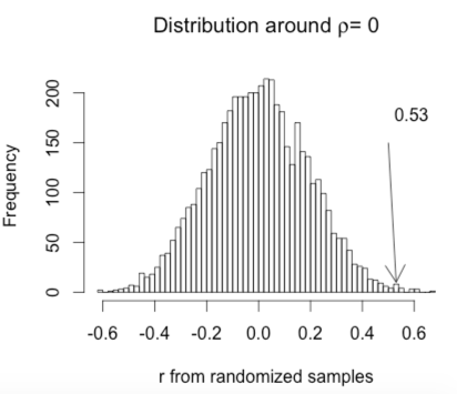
hist(r.random, breaks = 50, main = expression(paste("Distribution around ",rho, "= 0")), xlab = "r from randomized samples")
r.obt <- round(r.obt, digits = 2)
legend(.40, 200, r.obt, bty = "n")
arrows(.5,150,.53, 10)
____________________
The obtained correlation is 0.531767
Probability randomized r >= r.obt 0.002
 ____________________
Katz, S., Lautenschlager, G. J., Blackburn, A. B., & Harris, F. H. (1990) Answering reading comprehension items without passages on the SAT. Psychological Science, 1, 122-127.
![]()
dch: