

In some ways the randomization test on the means of two matched samples is even simpler than the corresponding test on independent samples. From the parametric t test on matched samples, you should recall that we are concerned primarily with the set of difference scores. If the null hypothesis is true, we would expect a mean of difference scores to be 0.0. We run our t test by asking if the obtained mean difference is significantly greater, or less than, than 0.0.
For a randomization test we think of the data just a little differently. If the experimental treatment has no effect on performance, then the Before score is just as likely to be larger than the After score as it is to be smaller. In other words, if the null hypothesis is true, a permutation within any pair of scores is as likely as the reverse. That simple idea forms the basis of our test.
One simple way to run our test is to imagine all possible rearrangements of the data between pre-test and post-test scores, keeping the pairs of scores together. We could create all of these possible rearrangements, each of which is equally likely if the null hypothesis of no treatment effect is true. For each of these rearrangements we could compute our test statistic, and then compare the statistic obtained from the original samples with the sampling distribution (I prefer to call it a reference distribution) we constructed by considering all rearrangements.
Life is actually even simpler than this. If we take the set of difference scores as our basic data, then rearranging pre- and post-test scores simply reverses the sign of the difference. So the easiest thing to do is to manipulate the sign of the difference, rather than the raw scores themselves. We can do this in many simple ways, but the simplest is to sample n scores from a distribution containing only +1 and -1. (In R this would simply be "signs <- sample(25, c(1,-1), replace = TRUE)"). Once we have done this we can multiply the vector of diffrence scores by the vector of signs to get a random arrangement of plus and minus signs on the difference scores. (e.g. "newsample <- signs*differences"). We can calculate our test statistic (in this case the mean) on that particular randomization sample. We can then repeat this nreps times, computing nreps statistics.
Everitt (1994) compared several different therapies as treatments for anorexia. one condition was cognitive behavior therapy, and he collected data on weights before and after therapy. These data are shown below.
cognitive behavior therapy
Before 80.50,  84.90,  81.50,  82.60,  79.90,  88.70,  94.90,  76.30,8  1.00,  80.50
After  82.20,  85.60,  81.40,  81.90,  76.40,  103.6,  98.40,  93.40,  73.40,  82.10

Before 85.00,  89.20,  81.30,  76.50,  70.00,  80.40,  83.30,  83.00,  87.70,  84.20
After  96.70,  95.30,  82.40,  72.50,  90.90,  71.30,  85.40,  81.60,  89.10,  83.90

Before 86.40,  76.50,  80.20,  87.80,  83.30,  79.70,  84.50,  80.80,  87.40,
After  82.70,  75.70,  82.60,  100.4,  85.20,  83.60,  84.60,  96.20,  86.70
Everitt was interested in testing the experimental hypothesis that cognitive behavior therapy would lead to weight gain. This comes down to testing the null hypothesis that the mean gain score is 0.0. The results of 5000 permutations of the data led to the following result. Here I have again used the mean gain as my metric.
The R code for this test is really quite short, although in the printout below I have deliberately lengthened it to show the various steps. The code can be downloaded at RandomMatchedSample/MatchedSample.r
#  Randomization Test on Matched Samples
#  Data from Everitt (1994)

#setwd("C:/Users/Dave/Dropbox/Webs/StatPages/ResamplingWithR/RandomMatchedSample")

dat <- read.table("http://www.uvm.edu/~dhowell/StatPages/ResamplingWithR/RandomMatchedSample/Everitt.dat", header = T)
diffObt <- mean(dat$After) - mean(dat$Before)
difference <- dat$After - dat$Before  #Use that order to keep most diff. positive

nreps <- 10000
set.seed(1086)
resampMeanDiff <- numeric(nreps)
for (i in 1:nreps) {
       signs <- sample( c(1,-1),length(difference), replace = T)
       resamp <- difference * signs
       resampMeanDiff[i] <- mean(resamp)
       }
       diffObt <- abs(diffObt)
highprob <- length(resampMeanDiff[resampMeanDiff >= diffObt])/nreps
lowprob <- length(dat$resampMeanDiff[dat$resampMeanDiff <= (-1)*dat$diffObt])/nreps
prob2tailed <- lowprob + highprob
cat("The probability from the sampling statistics is = ",prob2tailed,'\n')

hist(resampMeanDiff, breaks = 30, main = "Distribution of Mean Differences",
  xlab = "Mean Difference", freq = FALSE)
  text(1.5,.25,"Diff. obt")
  text(1.5,.23,round(diffObt,2))
  arrows(1.5, .21, diffObt, 0, length = .125)
  text(-3,.25,"p-value")
  text(-3,.23, prob2tailed)

  # Compare to Student's t
tvalue <- t.test(dat$Before, dat$After, paired = T)$statistic

cat("The t value from a standard matched-pairs t test is= ",tvalue, '\n')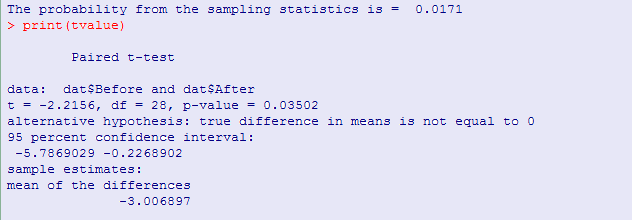
The result can also be seen in the histogram of the distribution of mean differences, which follows.
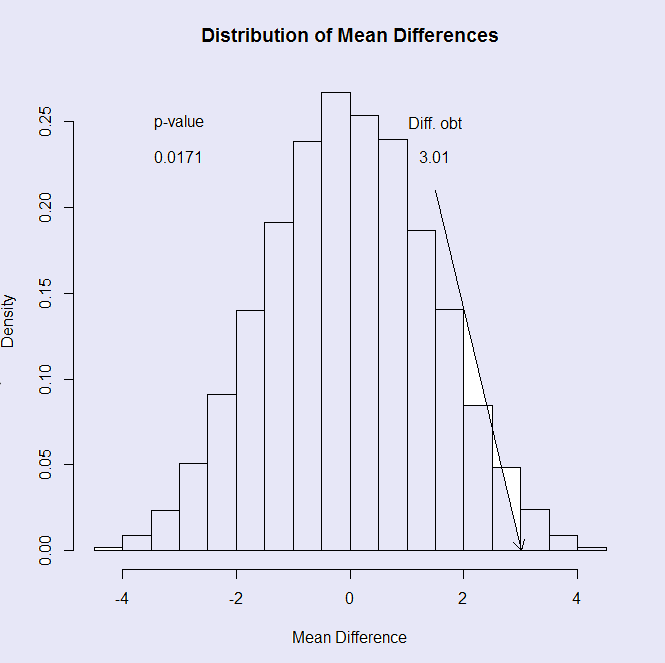
From the results you can see that the computed t value from the data was -2.216, with a p value of .035. Of the 10,000 different permutations, only 162 permutations gave a result as extreme as out sample mean difference, and so 1.62% of them led to a mean difference statistic as extreme as the one we found, so we can reject the null hypothesis and conclude that cognitive behavior therapy, or perhaps just the passage of time, did have an effect on weight (p = .016). The similarity, in this case, between the results of the resampling approach and the Student t approach illustrates Fisher's (1935) statement that only when the probability from the t distribution is similar to the probability from the resampling distribution, can we have faith in the t distribution's result.
You are probably going to get tired of seeing me bring up random assignment so often, but it is an important (actually a central) feature of randomization tests. Imagine a study that looks superficially like the one we just ran. Suppose that we have high-fat and a low-fat diet, and each participant lives on each diet for six months. At the end of each diet we weigh our subjects, and at the end of the study we compare the two groups' mean weights. In this study any careful investigator would randomly assign half of the subjects to have the high-fat diet followed by the low-fat diet, and the other half of the subjects would have the order reversed. In that situation we do have random assignment of treatment times, and we can draw meaningful conclusions. If the passage of time made a difference, it would help each group equally.
But the experiment that we actually analyzed in our example was different. For obvious reasons, all of our subjects had the pre-test measure followed by the post-test measure. There is no other sensible way of doing it. So we have not allowed for random assignment, and our conclusions are not as precise as we would like. The passage of time, and perhaps other variables that changed across the course of the experiment, independent of the treatment, are possible confounding variables. For that reason, I doubt that you would see this example in Edgington's book on randomization tests, because he takes a strict interpretation of the need for random assignment. But I suspect that most readers would be willing to conclude that there was a statistically significant increase in weight, even if we have to be a bit careful in attributing that to family therapy.
I don't wish to quarrel with Edgington, who has been a true believer in, and important advocate for, randomization tests from the beginning. And he deliberately, for theoretical reasons, takes a firm approach to random assignment. But I doubt that he would be willing to say that he has no idea if the students in his course even learned anything, because he can't randomly assign pre- and post-testing times. If they know more in December than they did in September, I hope that he would be willing to take some of the credit for that.
dch:
David C. Howell
University of Vermont
David.Howell@uvm.edu