

Superficially, a test on medians is similar to a test on means. But there are fundamental differences. With the two previous randomization tests (two independent samples and two paired samples), we saw that we could use the t computed between the means of two groups to measure differences. We don't have a t that we can use with medians, because we don't have a useful way of calculating the standard error, which is needed to compute a t. I chose the example that I will use particularly because a test on means and a test on medians come to very diferent conclusions. That does not usually happen, but I wanted to show that it does happen sometimes.
The simplest alternative statistic for such a test would be to take the obtained median difference as my statistic, and to count the number of randomizations that obtained a median difference as great as the one in our obtained data. There are other alternatives, but that is the one that I will use here.
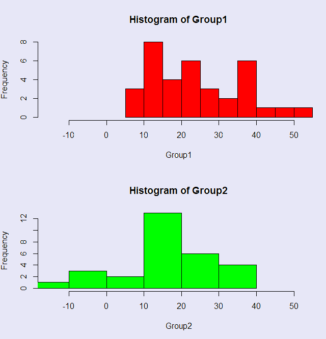
I will use an example from Adams et al on sexual arousal and homophobia. This example measures sexual arousal in homophobic and nonhomophobic participants and shows, interestingly, that the homophobic males are more sexually aroused by watching a video of homosexual behavior. At least that is clearly what you find with a t test or a randomization test on means. We will find quite a different answer when we compare medians, though it is hard to explain why.The data are available at Tab7-5. The R code for this analysis is available at MedianDifference.r. It is worth looking at the code because I have added some extra material near the end to go along with some of the comments below. I have plotted histograms of the two groups so that you can see the overlap in their distributions. There is considerable overlap, suggesting that perhaps the groups do not differ significantly.
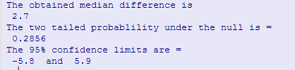
I created 5000 random permutations of the 35 + 29 = 64 observations. For each permutation the first 35 scores were assigned to the Homophobic condition, and the last 29 observations to the Nonhomophobic condition. I then calculated the median under each condition, and then the median difference. Across 5000 resamples, this gave me the sampling distribution of the difference between two medians. I then calculated a two-tailed probability by counting the number of those differences that exceeded the absolute value of the obtained median difference in the samples. For this particular run the resulting two-tailed p value was .2904. I also estimated something that looks like confidence limits, but really are not. By taking the 2.5% and 97.5% limits for the distribution of differences for randomized samples, I find that 95% of the distribution of median differences fall between -5.8 and 6.0. BUT these are not standard confidence limits. These tell you that if the null hypothesis is true, 95 % of the median differences would fall in that interval. We are roughly taking the cutoffs for 47.5% of the observations above and below a null difference of 0. In other words, these limits on centered on 0, not on the obtained median difference. So I would hesitate to call them confidence limits. They are more like null limits.
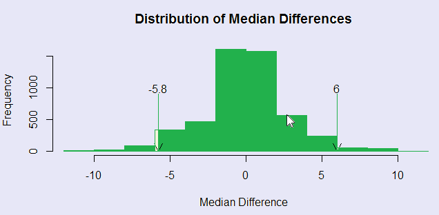
The results of this approach in terms of the distributions of medians can be seen in the following figure. Notice that the differences in medians when there is no difference between treatments seem to range from roughly -5 to 5. (The "null limits" are -5.8 to 6.0.) Our obtained median difference was 2.7, which falls under the bulk of the distribution. The printout from R is also shown.
Notice that this sampling distribution is noticeably more sparse than the distributions we have seen for means. That is because of the limited possibilities for a median. It must either be one of the values in the original sample, or half way between two original values.
A second, and very important, point is that there is a major difference, for these data, between the test on the medians and the results of a standard test on the means (either a t-test or the result of randomizing mean differences.) The probability under the null that we found here was .2856 (probabilities vary somewhat from one run to another.) Another program for resampling medians gave me a probability of .308. If we ran a t test, the probability would only be .01547. When I created a randomization test on the means, I found a p value of .0128, which is certainly in line with the t test. In other words, for this example there is a huge difference between testing means and testing medians. It was such a great difference that I doubted it at first. But it is in line with what I would get running a Wilcoxon's test (p = .315), which is a randomization test randomizing the ranked data, rather than the raw data. So I guess I'm right.
A very complete set of resampling tests can be found in the "coin" package, where "coin" stands for "conditional inference." This package is not always easy to use because the help pages are not as helpful as they could be. A good discussion of this package can be found in Kabacoff (R In Action, 2011). (I found part of that discussion on line, though it is a broader discussion than the example given here.) But the interesting thing about the coin package is that the "median_test" function is a rank randomization test, permuting the ranks rather than the observations. Two different data sets having the same ranked data but different numerical data give the same probability under the median_test, though quite different results when in my code.
This could be expanded to multiple groups, but I have not yet thought what a good test statistic would be. I would suggest trying the test statistic (H) for the Kruskal-Wallis test, but use the raw scores instead of the ranks. I haven't tried it, so I make no promises.
![]()
dch:
David C. Howell
University of Vermont
David.Howell@uvm.edu