


This page focusses on a variety of designs having repeated measures. Some of these designs also have between subject measures. It is my hope that you will be able to take a particular set of code and adapt it to your own needs.
Even without randomization, the repeated measures analysis of variance using R is somewhat more complicated that most analyses of variance. For a discussion of those tests, you can go to . An excellent discussion of alternative ways of dealing with repeated measures anova in R can be found at https://gribblelab.wordpress.com/2009/03/09/repeated-measures-anova-using-r/.
Just as we did with the one-way analysis of variance on independent samples, we will use the normal F statistic. It summarizes the differences between means, and eliminates the effects of between-subjects variability.
With repeated measures, we want to permute the data within a subject, and we don't care about between-subject variability. If there is no effect of treatments or time, then the set of scores from any one participant can be exchanged across treatments or time. In what follows I will assume that the repeated measure is over time, though there is no restriction that it need be.
The following example is loosely based on a study by Nolen-Hoeksema and Morrow (1991). The authors had the good fortune to have measured depression in college students two weeks before the Loma Prieta earthquake in California in 1987. After the earthquake they went back and tracked changes in depression in these same students over time. The following example is based on their work, and assumes that participants were assessed every three weeks for five measurement sessions.
I have changed the data from the ones that I have used elsewhere to build in a violation of our standard assumption of sphericity. I have made measurements close in time correlate highly, but measurements separated by 9 or 12 weeks correlate less well. This is probably a very reasonable thing to expect, but it does violate our assumption of sphericity.
If we ran a traditional repeated-measures analysis of variance on these data we would find
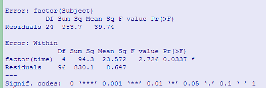
Notice that Fobt = 2.726, which is significant, based on unadjusted df, with p = .034. Greenhouse and Geisser's correction factor is 0.617, while Huynh and Feldt's is 0.693. Both of these lead to an increase in the value of p, and neither is significant at a = .05. (The F from a multivariate analysis of variance, which does not require sphericity has p = .037.)
We can apply a randomization test to these data using the code shown below. This code may be harder to read than most. That is because I had a lot of trouble coming up with a way of randomizing the time measurements within subjects. I finally did it, but it takes a bit of thinking. The code also produces a standard analysis of variance table. The "Error: factor(Subject)" section just tells you about the variability among subjects, which is not particularly interesting. The "Error:Within" section tests the time (or trials) factor and is what we mainly want.
#  R for repeated measures
#  One within subject measure and no between subject measures
#  Be sure to run this from the beginning because
#  otherwise vectors become longer and longer.
library(car)
rm(list = ls())
  ##  You want to clear out old variables --with "rm(list = ls())" --
  ##  before building new ones.
data <- read.table(("http://www.uvm.edu/~dhowell/StatPages/ResamplingWithR/
RandomRepeatMeas/NolenHoeksema.dat"), header = TRUE)

datLong <- reshape(data = data, varying = 2:6, v.names = "outcome", timevar
= "time", idvar = "Subject", ids = 1:9, direction = "long")

datLong$time <- factor(datLong$time)
datLong$Subject <- factor(datLong$Subject)
orderedTime <- datLong[order(datLong$time),]
options(contrasts=c("contr.sum","contr.poly"))
modelAOV <- aov(outcome~factor(time)+Error(factor(Subject)), data = datLong)
print(summary(modelAOV))
obtF <- summary(modelAOV)$"Error: Within"[[1]][[4]][1]

par( mfrow = c(2,2))
plot(datLong$time, datLong$outcome, pch = c(2,4,6), col = c(3,4,6))
legend(1, 20, c("same", "different", "control"), col = c(4,6,3),
                      text.col = "green4",  pch = c(4, 6, 2),
                       bg = 'gray90')
nreps <- 1000
counter <- 0
Fsamp <- numeric(nreps)

times <- c(1:5)
permTimes <-NULL

for (i in 1:nreps) {
for (j in 1:25) {
  permTimes <- c(permTimes, sample(times,5,replace = FALSE))
  }
orderedTime$permTime <- permTimes
sampAOV <- aov(outcome~factor(permTime)+Error(factor(Subject)), data = orderedTime)
Fsamp[i] <- summary(sampAOV)$"Error: Within"[[1]][[4]][1]
if (Fsamp[i] > obtF) counter = counter + 1
permTimes <- NULL
}

p <- counter/nreps
cat("The probability of sampled F greater than obtained F is = ", p, '\n')
 hist(Fsamp, breaks = 50, bty = "n")
 legend(1.5,50,bquote(paste(p  == .(p))), bty = "n" )

THE RESULTS FOLLOW:

Error: factor(Subject)
          Df Sum Sq Mean Sq F value Pr(>F)
Residuals 24    954    39.7

Error: Within
             Df Sum Sq Mean Sq F value Pr(>F)
factor(time)  4     94   23.57    2.73  0.034 *
Residuals    96    830    8.65
---
Signif. codes:  0 ‘***’ 0.001 ‘**’ 0.01 ‘*’ 0.05 ‘.’ 0.1 ‘ ’ 1

FROM THE RANDOMIZATION TEST WE OBTAIN:
The mean F from randomization is 0.85.
The probability of sampled F greater than obtained F is =  0.013.
Having two repeated measures is not really much different than having one. Instead of each subjects data across the one measure, we will randomize it across the second measure as well. For example, if we had a 2 X 5 design, both measures being repeated, each subject would have 10 scores and those 10 scores would be randomized.
This question was raised in an e-mail from Ben Bauer at the University of Trent in Canada. I am grateful to him for showing me the simple way, which I could not for some reason figure out, to randomize the data. (My way worked, but it was more on the brute-force end.)
The data are taken from a study by Bouton and Swartzentruber (1985) on conditioned suppression, but I have only used the data from Group 2. (This study is discussed in my book on Statistical Methods for Psychologists, 8th ed.) on page 484ff. In this study each of 8 subjects was measured across two cycles on each of 4 phases, so Cycle and Phase are repeated measures. The code is shown below.
################################################################################# Randomization Test for Two Within-Subject Repeated Measures ### One tricky part of this code came from Ben Bauer at the Univ. of Trent, Canada. ###He writes code that is more R-like than I do. In fact, he knows more about R than ###I do. # Two within subject variables, 1:8 # Data from Bouton & Schwartzentruber (1985) -- Group 2 # Methods8, p. 486 data <- read.table("http://www.uvm.edu/~dhowell/methods8/DataFiles/ Tab14-11long.dat", header = T) n <- 8 #Subjects cells <- 8 #cells = 2*4 nobs <- length(data$dv) attach(data) cat("Cell Means \n") print(tapply(dv, list(Cycle,Phase), mean)) #cell means cat("\n") Subj <- factor(Subj) Phase <- factor(Phase) Cycle <- factor(Cycle) #Standard Anova options(contrasts = c("contr.sum","contr.poly")) model1 <- aov(dv ~ (Cycle*Phase) + Error(Subj/(Cycle*Phase)), contrasts = contr.sum) summary(model1) # Standard repeated measures anova table <- (summary(model1)) # Extracting obtained F values cycle <- table[[2]] F.cycle.obt <- cycle[[1]][[4]][[1]] phase <- table[[3]] F.phase.obt <- phase[[1]][[4]][[1]] cxp <- table[[4]] F.cxp.obt <- cxp[[1]][[4]][[1]] #Now I have stored away the obtained F values # Beginning of randomization test nreps <- 1000 FR.cycle <- numeric(nreps) FR.phase <- numeric(nreps) FR.cxp <- numeric(nreps) for (i in 1:nreps) { randomdv <- NULL for (j in seq(from=1, to=nobs, by=8) ) { randomdv <- c(randomdv,sample(dv[j:(j+7)])) } modelrandom <- aov(randomdv ~ (Cycle*Phase) + Error(Subj/(Cycle*Phase)), contrasts = contr.sum) summary(modelrandom) table <- (summary(modelrandom)) # Extracting F values on randomized data # table # table[[1]] cycle <- table[[2]] FR.cycle[i] <- cycle[[1]][[4]][[1]] phase <- table[[3]] FR.phase[i] <- phase[[1]][[4]][[1]] cxp <- table[[4]] FR.cxp[i] <- cxp[[1]][[4]][[1]] } probCycle <- length(FR.cycle[FR.cycle >= F.cycle.obt])/nreps cat("prob for Cycle = ", probCycle, "\n") probPhase <- length(FR.phase[FR.phase >= F.phase.obt])/nreps cat("prob for Phase = ", probPhase, "\n") probCXP <- length(FR.cxp [FR.cxp >= F.cxp.obt])/nreps cat("prob for interaction = ", probCXP, "\n")Output
Cell Means 1 2 3 4 1 17.750 22.375 23.125 20.25 2 20.875 28.125 20.750 24.25 TRADITIONAL ANOVA Error: Subj Df Sum Sq Mean Sq F value Pr(>F) Residuals 7 8411 1202 Error: Subj:Cycle Df Sum Sq Mean Sq F value Pr(>F) Cycle 1 110.2 110.25 2.877 0.134 Residuals 7 268.2 38.32 Error: Subj:Phase Df Sum Sq Mean Sq F value Pr(>F) Phase 3 283.4 94.46 1.029 0.4 Residuals 21 1928.1 91.82 Error: Subj:Cycle:Phase Df Sum Sq Mean Sq F value Pr(>F) Cycle:Phase 3 147.6 49.21 0.728 0.547 Residuals 21 1418.9 67.57 PROBABILITIES FROM RANDOMIZATION TEST prob for Cycle = 0.136 prob for Phase = 0.424 prob for interaction = 0.513
### Randomization Test for Two Within-Subject Repeated Measures
 and one between-subject measure

# Data from Bouton & Schwartzentruber (1985) --
# Methods8, p. 486

rm(list = ls())
data <- read.table("http://www.uvm.edu/~dhowell/methods8/DataFiles/Tab14-11.dat",

 header = T)
attach(data)
Phase <- factor(rep(1:2, each = 24, times = 4))
Cycle <- factor(rep(1:4, each = 48))
Group = factor(rep(1:3, each = 8,times = 8))
dv <- c(C1P1, C1P2, C2P1, C2P2, C3P1, C3P2, C4P1, C4P2)
Subj <- factor(rep(1:24, times = 8))
n <- 24    #Subjects
withincells <- 8    #withincells = 2*4
nobs <- length(dv)

cat("Cell Means Across Subjects \n")
print(tapply(dv, list(Cycle,Phase), mean))    #cell means
cat("\n")
#Standard Anova
options(contrasts = c("contr.sum","contr.poly"))
model1 <- aov(dv ~ (Group*Cycle*Phase) + Error(Subj/(Cycle*Phase)),
  contrasts = contr.sum)
print(summary(model1))   # Standard repeated measures anova

table <- (summary(model1))   # Extracting random F values
group <- table[[1]]
F.group.obt <- table[[1]][[1]][[4]][[1]]
cycle <- table[[2]]
F.cycle.obt <- cycle[[1]][[4]][[1]]
F.CG.obt <- cycle[[1]][[4]][[2]]
phase <- table[[3]]
F.phase.obt <- phase[[1]][[4]][[1]]
F.PG.obt <- phase[[1]][[4]][[2]]
cxp <- table[[4]]
F.CP.obt <- cxp[[1]][[4]][[1]]
F.CPG.obt <- cxp[[1]][[4]][[2]]
#Now I have stored away the obtained F values

# Beginning of randomization test

nreps <- 5000
F.group.ran <- numeric(nreps)    # Vectors to store F values
F.cycle.ran <- numeric(nreps)
F.CG.ran  <- numeric(nreps)
F.phase.ran <- numeric(nreps)
F.PG.ran  <- numeric(nreps)
F.CP.ran <- numeric(nreps)
F.CPG.ran <- numeric(nreps)
for (i in 1:nreps) {
   randomdv <- NULL
   for (j in seq(from=1, to=nobs, by=8) ) {
      randomdv <- c(randomdv,sample(dv[j:(j+7)])) }
   step1 <- rep(1:3, each = 8); step2 <- sample(step1, 24, replace = FALSE)
   step3 <- rep(step2, times = 8)
   Grp <- step3      # Randomizing Group variable
   modelrandom <- aov(dv ~ (Grp*Cycle*Phase) + Error(Subj/(Cycle*Phase)),
     contrasts = contr.sum)

   summary(modelrandom)

   table2 <- (summary(modelrandom))   # Extracting obtained F values
   group <- table2[[1]]
   F.group.ran[i] <- table2[[1]][[1]][[4]][[1]]
   cycle <- table2[[2]]
   F.cycle.ran[i] <- cycle[[1]][[4]][[1]]
   F.CG.ran[i] <- cycle[[1]][[4]][[2]]
   phase <- table2[[3]]
   F.phase.ran[i] <- phase[[1]][[4]][[1]]
   F.PG.ran[i] <- phase[[1]][[4]][[2]]
   CP <- table2[[4]]
   F.CP.ran[i] <- CP[[1]][[4]][[1]]
   F.CPG.ran[i] <- CP[[1]][[4]][[2]]
}
probGroup <- length(F.group.ran[F.group.ran >= F.group.obt])/nreps
cat("Prob for Group = ", probGroup, "\n")
probCycle <- length(F.cycle.ran[F.cycle.ran >= F.cycle.obt])/nreps
cat("Prob for Cycle = ", probCycle, "\n")
probCG <- length(F.CG.ran[F.CG.ran >= F.CG.obt])/nreps
cat("Prob for Cycle by Group = ", probCG, "\n")
probPhase <- length(F.phase.ran[F.phase.ran >= F.phase.obt])/nreps
cat("Prob for Phase = ", probPhase, "\n")
probPG <- length(F.PG.ran[F.PG.ran >= F.PG.obt])/nreps
cat("Prob for Phase by Group = ", probPG, "\n")
probPC <- length(F.CP.ran[F.CP.ran >= F.CP.obt])/nreps
cat("Prob for Phase by Cycle ",probPC,"\n")
probCPG <- length(F.CPG.ran[F.CPG.ran >= F.CPG.obt])/nreps
cat("Prob for Phase by Cycle by Group ",probCPG,"\n")
 <.pre>
Things become a bit messier when we have a design with both between and within subject measures. When there are only between measures, you can randomize across groups. When there are only repeated measures, you can randomize within subjects. But what do you do when you have both. My solution was to first randomize within subjects. I then take those as my "raw data" and randomize them across groups. That gives me results that seem reasonable, and the logic seems perfectly reasonable to me.
I am going to use an example of a study with one between subject measure and one within subject measure, I am then going to extend that to one between and two within subject measures.
# This was originally written by Joshua Wiley, in the Psychology Department at UCLA.
#  Modified for one between and one within for King.dat by dch

### Howell Table 14.4 ###
## Repeated Measures ANOVA with 2 variables
## Read in data, convert to 'long' format, and factor()
dat <- read.table("http://www.uvm.edu/~dhowell/methods8/DataFiles/
Tab14-4.dat", header = TRUE)
head(dat)
dat$subject <- factor(1:24)
datLong <- reshape(data = dat, varying = 2:7, v.names = "outcome", timevar
= "time", idvar = "subject", ids = 1:24, direction = "long")
datLong$Interval <- factor(rep(x = 1:6, each = 24), levels = 1:6, labels = 1:6)
datLong$Group <- factor(datLong$Group, levels = 1:3, labels = c("Control",
"Same", "Different"))
cat("Group Means","\n")
cat(tapply(datLong$outcome, datLong$Group, mean),"\n")
cat("\nInterval Means","\n")
cat(tapply(datLong$outcome, datLong$Interval, mean),"\n")
# Actual formula and calculation
King.aov <- aov(outcome ~ (Group*Interval) + Error(subject/(Interval)), data = datLong)
# Present the summary table (ANOVA source table)
print(summary(King.aov))
interaction.plot(datLong$Interval, factor(datLong$Group),
 datLong$outcome, fun = mean, type="b", pch = c(2,4,6),
  legend = "F",
  col = c(3,4,6), ylab = "Mean of Outcome",
  legend(4, 300, c("Same", "Different", "Control"), col = c(4,6,3),
                      text.col = "green4", lty = c(2, 1, 3), pch = c(4, 6, 2),
                      merge = TRUE, bg = 'gray90')
# Two between subject variables, one within
# Data from St. Lawrence et al.(1995)
# Methods8, p. 479

#  Note: In data file each subject is called a Person, and I convert that to a factor.
# In reshape, it creates a variable called "subject," but that is not what I want to use.
#  In aov the model is based on Person, not subject.
rm(list = ls())
data <- read.table("http://www.uvm.edu/~dhowell/methods8/DataFiles/
Tab14-7.dat", header = T)
head(data)
# Create factors
data$Condition <- factor(data$Condition)
data$Sex <- factor(data$Sex)
data$Person <- factor(data$Person)
#Reshape the data
dataLong <- reshape(data = data, varying = 4:7, v.names = "outcome", timevar
= "Time", idvar = "subject", ids = 1:40, direction = "long")
dataLong$Time <- factor(dataLong$Time)

tapply(dataLong$outcome, dataLong$Sex, mean)
tapply(dataLong$outcome, dataLong$Condition, mean)
tapply(dataLong$outcome, dataLong$Time, mean)
options(contrasts = c("contr.sum","contr.poly"))
model1 <- aov(dataLong$outcome ~ (dataLong$Condition*dataLong$Sex*
factor(dataLong$Time)) + Error(dataLong$Person/(dataLong$Time)))
summary(model1)
Last revised: 6/29/2025