

This page preesents a variety of graphical demonstrations that are programmed in R. The original source of many of these is related to a paper by Bowman, Crawford, Alexander, & Bowman (2007) Although they are written in R, you do not need to know much about R in order to run them. In fact, the first part of this document duplicates other pages and relates to how to get R (it is free), how to install it, and how to run it. I no longer have a Macintosh, so I can't speak authoritatively about running R on a Mac, but there is plenty of help on the R site (http://cran.r-project.org/) to handle any problems that are likely to arise. Well, now I do have a Mac. There is almost no difference between a Mac and a PC as far as R is concerned. But there is one thing that you shoud pay attention to. Macs used to have something called X11, (or XQuartz) to do graphics. The newest machines no long have it. But you can download it easily from the XQuartz site , and it installs easily. You may have to start it up before you start R for the first time. Also, if you are running a very old Windows machine with Vista, you should probably do a quick Google search to check out any problems.
In some ways this age is more advanced than an introduction should be. But on the other hand, it is written primarily to show you the kinds of things that are possible, with no particular intent to teach you the underlying code. That will come later. I just want you to get a sense of the range of things that are possible.
I assume that you have R running, but if not, start it. I hate texts that think you are so dim that you will be all excited when you can make your computer type "Hello, World." (Unix people love to start that way, and then they talk about foo and foobar--that's how you know they are Unix people. Its like someone who says "Dude" over and over again; they are probably a Colorado snowboarder.) We are going to start with something a great deal more interesting--at least I think so. We are going to plot a regression line and then fiddle with it. Then we are going to move to three dimensional surfaces. The data that I am using can be found at the Web site for my "Methods" book and is named "albatros.dat." (It relates to data from a course by course student evaluation of teaching.) You can either download that or make up your own. If you download that file, stick it someplace where you will remember it, such as in a folder called "R Stuff." The folder can be called anything you like, but it will be best if you keep all the files that I will talk about here in that same folder. That data file has six variables, but I will only play with three because that is all I need. But first we have to read in the data.
Because you have R running, you can go to the R console and type in
the following commands. (We'll see later how to enter them into a file
and submit that, but for now every command (well most) will execute as
you enter them.) The rpanel library is a library of useful graphical functions.
 install.packages("rpanel")  #necessary if you have not already installed it.
library(#rpanel")                   #the rgl package is also required, but it will be loaded automatically
data <- read.table(file.choose(), header = TRUE)    #Use Albatros.dat in fundamentals8
# or
data <- read.table("http://www.uvm.edu/~dhowell/fundamentals8/DataFiles/albatros.dat")
attach(data)
Something that is going to drive you crazy is the fact that R is case sensitive. That means that the word "this" starting with a capital letter is completely and utterly different from "this" starting with a lower case letter. That goes way back to the origins of R, which began at Bell Labs and was called S. (I guess they liked short names!) S transmogrified into R and into S-Plus, which are almost the same except that S-Plus costs real money, if you can find it, while R is free. There are a few commands that work differently in the two languages, but very few.
The first command loads that package that you just downloaded, called rpanel. When you installed it, you only made it available if called. The "library(rpanel)" actually tells it to wake up and get ready to do something. The second command will open up a dialog window so that you can go hunting for the data file that you so carefully saved. After you get the data you can see the data file by entering head(data) and you will see the beginning of the dataset. Adding the word "head" simply tells it to only write out a few lines, rather than scrolling the interesting stuff off the page.
Contrary to what you might think, you really don't have a variable named "Teach" readily available to you. It is part of a data file (called a data.frame) named "data" and you would have to call it as data$Teach, which quickly becomes a pain in the neck. So the "attach" command yanks a copy of Teach out of the data set and makes it available for you to call by its very own name. But I strongly recommend that you look at attach.html first
Just to show you want R can do, we will make use of some of its built in functions. For example, if you type "mean(Teach)" (without the quotation marks) it will spit out the mean value for Teach. You can probably guess what will happen if you type "sd(Teach)" or var(Teach). You can go further by typing "cor(Teach, Knowledge, Overall)" This will give the set of correlations between each of those variables taken two at a time. There is a good bit that you can do like this without knowing a lot about R. We are about to do something like that but a lot more fancy. But our commands won't be noticeably longer.
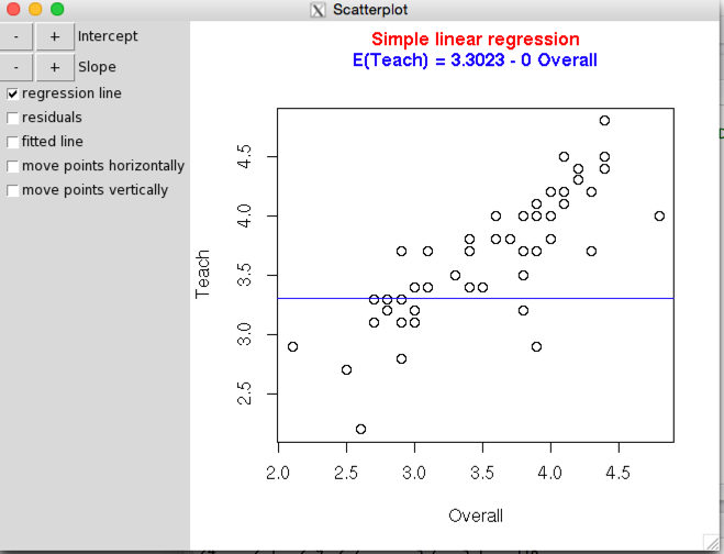
Let's start by just plotting Overall against Teach. Since Overall is the overall student rating of an instructors performance, and Teach is a rating of his or her teaching skills, it makes sense to use Overall as the dependent variable. Because you have loaded the rpanel library you have the command rp.regression(Overall, Teach)
available to you. Just type that at the prompt. You will get the following result, or something like it.
The most obvious thing that you see there is a scatterplot, but the interesting stuff is in the upper left. There you can click on the + and - to increase or decrease the intercept, and you can do the same to vary the slope. As these change, so does the equation above the scatterplot. You can play with these controls to move the line up or down and change its slope until you have a line that looks like it goes through the data just as the true regression line will. Then you can move down a bit and click on the box ("fitted line") that displays the optimal regression line and see how close you came. Finally, you can move down a bit lower and click on boxes that will allow you to move individual data points left to right or up and down. You will see how the regression line changes as you move the points. (The point springs back to its original location when you release the mouse.
We can do one better than the previous demonstration by using another function called rp.regression2. That function will take three variables as input and plot them in three-dimensional space. You can then move the space around and see what it looks like. This is the same figure, more-or-less, that you see in Figure 15.1 in my book. The command is remarkably simple, especially considering how much it is doing. You simply enter rp.regression2(Overall, Teach, Knowledge) (Don't try to be cute by adding all three variables to the previous (rp.regression()) command. It just makes an awful mess. The figure below is what you will get, although you may have to use your mouse to move the various bits around so that you can see them.
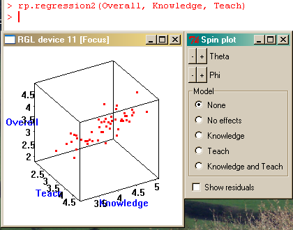
As you can see, there are a bunch of things that you can do with this plot. Theta and Phi allow you to rotate it in three-dimensional space. In addition, You can ask it to plot the regression of Overall on either Teach or Knowledge, or on both. Notice how the plane through the points changes as you change the predictors.
Well, first of all you could substitute variable names and use other variables in this data set. That will get old soon. Alternatively, you can use this same function and play with your own data. Simply make up a data file in three (or more) columns with the variable names in the first row. Then load it just as you did the one above.
But there is more that you can do even with these variables. Entering
the following commands will allow you to look at the individual
variables and plot them in different ways.
var.plot <- Teach
density.draw <- function(panel) {
  plot(density(panel$x, bw = panel$h), main = "Density")
  panel
  }

data.plotfunction <- function(panel) {
   if (panel$plot.type == "histogram")
      hist(panel$x, main = "Histogram")
   else
      if (panel$plot.type == "boxplot")
        boxplot(panel$x, main = "Boxplot")
   else
     density.draw(panel)
     panel
   }

panel <- rp.control(x = var.plot)
rp.listbox(panel, plot.type, c("histogram","boxplot","density estimate"),
action = data.plotfunction, title = "Plot type")
rp.slider(panel, h, 0.1, 5, log = TRUE, action = density.draw)
The simplest way to do this is to simply cut and paste these commands into a text file, and then paste them into R. (There are better ways, but this will do.) You will notice that the first line of the script sets var.plot <- Teach. By changing that to a different variable name you can work with each of your variables. (I tried to create a dialog box to do that for you, but I gave up. It isn't that it couldn't be done, it's that I'm not smart enough (yet) to do it.). If you submit this code you will get something like the following.
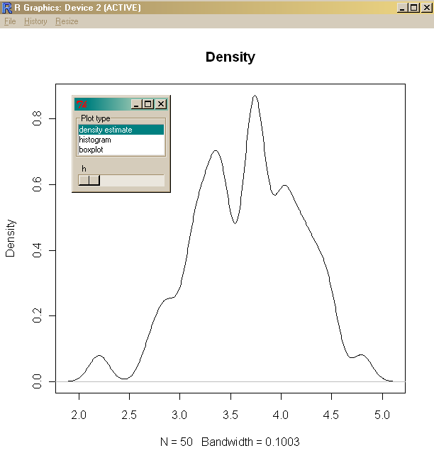
I moved things around before cutting and pasting the figure, and you may want to also. The first plot that you see is a density plot, which is a way of fitting a curve to data so as to be faithful to the true wiggles in the plot and to play down noise. (The 7th edition of my "Methods" book discusses density plots.) Think of it as taking a weighted average of the heights of nearby points as you move across the figure. In the little box you will see a slider labeled "h." If you move that left and right you will change the bandwidth that is used to draw a particular section of the curve, and as you make the bandwidth larger the curve will smooth out. After you get bored looking at that you can click on "histogram" or "boxplot" and get different views of the variable.
So far we have only used two of the functions that Bowman et al. provided. But there are a lot more. My suggestion is to type ?rpanel
at the R prompt. This will give you the help files that go with this package. Help files in R are not noted for the warm fuzzy hands-on help that you might like, but they are generally helpful. The file that you will start out with looks like
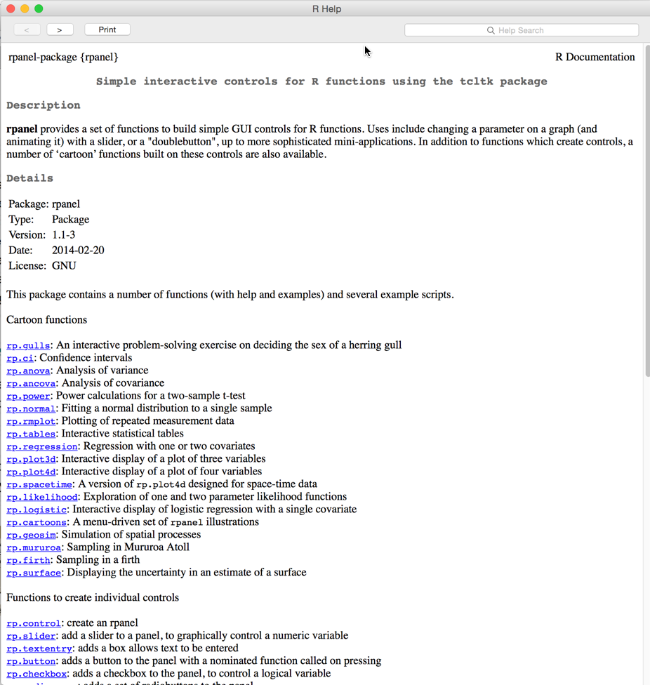
Over at the left you will see a list of all of the parts of the
package. And by clicking on each of those functions you will put up a
new help page. Part way down you will see something named rp.logistic, and it's a good
bet that it deals with logistic regression. I'm choosing this because I
have not played with it before, so both of us get to learn how to use
it. I am certainly likely to need a data file, so I have made one
available at survdata.dat
This relates to whether or not a person survived a diagnosis of cancer
as a function of the survival rating his/her doctor gave at the time of
diagnosis. You can forget all variables except outcome and survrate.
Load the data by typing
survdata <- read.table(file.choose(), header = TRUE)
at the prompt.) Near the top of the help file you will see rp.logistic(x, y, xlab = NA, ylab = NA, panel.plot = TRUE,hscale = NA, vscale = hscale)
I bet that the x and y refer to the data, which in our terms would be survrate and outcome. "xlab" and "ylab" are the axis labels, and NA means that the default is "not available." We don't know what panel.plot is, though there is a brief description a bit lower, so we will take the default. "hscale and vscale are going to refer to the size of the plot, so we might as well take the defaults again. So our command seems to come down to rp.logistic(survrate, outcome) at least we will start from there. rp.logistic(survrate, outcome) Error in rp.logistic(survrate, outcome) : object "outcome" not found.
Oops! I forgot to attach(survdata) so it couldn't find my variables.
attach(survdata)
rp.logistic(survrate, outcome)
Wow! It worked! At least I got a figure. And if I play with alpha and beta I can get a plot that looks vaguely like like the one in my book (in 6th edition it was Figure 15.9). You can do even better if you click on "fitted model." If I want to spice it up I could replace the xlab = NA with something like xlab = Predicted Survival Rate
Oops, that didn't work so put the label itself in quotation marks. xlab = "Predicted Survival Rate"
We could change hscale and vscale, but the help file doesn't give us a lot of advice on what kind of numbers to use. So I tried 1 and 2, respectively, and got a tall skinny thing. Well, at least I get the general idea, and could play further.
Playing with the left side of the help screen I came to something called rp.power, and I suspect that it refers to power analysis. When I ask for the help screen I get rp.power(). That's odd, it doesn't have anything between the (), which means that I don't need to pass it any variables. So just try rp.power()
That gave me a graph and a little dialog box asking me to supply (increase or decrease) n, mu1, mu2, and sigma. When I do I see how the power varies as a function of these values. I also have a little box that I can check to see a plot of the two populations superimposed. Not bad.
First of all, there are a lot of things here to play with and keep yourself busy. But if you want to learn a bit about R, you can then create your own functions. If you want to learn R, I personally think that Crawley's book, with the very creative title of "The R Book," is perhaps the best. Moreover, if you issue a function call without any (), you will see the program statements themselves. For example, if you type rp.cartoons() you will find a very good set of functions that you can run just by choosing from a dropdown menu. (Don't be put off by the silly name.) And if you type rp.cartoons without the parentheses, you will see all of the code. If you see something that you almost like, steal the code (giving credit, please), modify it, and come up with something closer to what you want. This code is all open software, so you really are allowed to take someone elses code and modify it. But PLEASE give them credit.
Oh, and I almost forgot. Go to Google and type rpanel. You will find a lot of the stuff referred to above and some other goodies. Never underestimate Google -- or trust them!
rpanel is not the only graphical interface available in R. There is also "playwith," and you can download those functions just like you downloaded rpanel. It is also worth a look.
Bowman, A., Crawford, E., Alexander, G., & Bowman, R. W. (2007) rpanel: Simple interactive controls for R functions using the tcltk package. Journal of Statistical Software, 17, 1-18. (This paper is available on the web via a simple Google search.)
Crawley, M. J. (2007) The R Book. Chichester, England: Wiley.

dch:
David C. Howell
University of Vermont
David.Howell@uvm.edu