

In some ways, a one-way analysis of variance using R is straightforward and doesn't take a lot of work to set up. If fact, it can be very simple. But then we can add complications by using contrasts, either orthogonal or nonorthogonal, using post-hoc tests, and moving to a more complex design. On top of that, the approach looks as if we are using mutiple regression to perform our analysis, whereas with something like SPSS you use a procedures called Anova. Actually, the distinction is not as real as it looks. This page will start off with the simplest approach and expand on that as we go along.
We will begin with a simple data set out of one of my texts. The example comes from a study by Siegel (1975) on morphine tolerance. To quote from the text, "At the simplest level he placed mice on a warm surface and simply noted how long it took for them to lick their paws. Siegel noted that there are a number of situations involving drugs other than morphine in which conditioned (learned) drug responses are opposite in direction to the unconditioned (natural) effects of the drug. For example, an animal injected with atropine will usually show a marked decrease in salivation. However if physiological saline (which should have no effect whatsoever) is suddenly injected (in the same physical setting) after repeated injections of atropine, the animal will show an increase in salivation. It is as if the animal were expecting atropine, and thus doing something to make his body compensate for what he things is coming. In such studies, it appears that a learned compensatory mechanism develops over trials and counterbalances the effect of the drug."
Siegel theorized that such a process might help to explain morphine tolerance. He reasoned that if you administered a series of pretrials in which the animal was injected with morphine and placed on a warm surface, morphine tolerance would develop. Thus, if you again injected the subject with morphine on a subsequent test trial, the animal would only be as sensitive to pain as would be a naive animal (one who had never received morphine) because of the tolerance that has fully developed. Siegel further reasoned that if on the test trial you instead injected the animal with physiological saline in the same test setting as the normal morphine injections, the conditioned hypersensitivity that results from the repeated administration of morphine would not be counterbalanced by the presence of morphine, and the animal would show very short paw-lick latencies and heighten sensitivity. Siegel also reasoned that if you gave the animal repeated morphine injections in one setting but then tested it with morphine in a new setting, the new setting would not elicit the conditioned compensatory hypersensitivity to counterbalance the morphine. As a result, the animal would respond as would an animal that was being injected for the first time. Heroin is a morphine derivative. Imagine a heroin addict who is taking large doses of heroin because he has built up tolerance to it. If his response to this now large dose were suddenly that of a first-time (instead of a tolerant) user, because of a change of setting, the result could be, and often is, lethal. We're talking about a serious issue here, and drug overdoses often occur in novel settings.
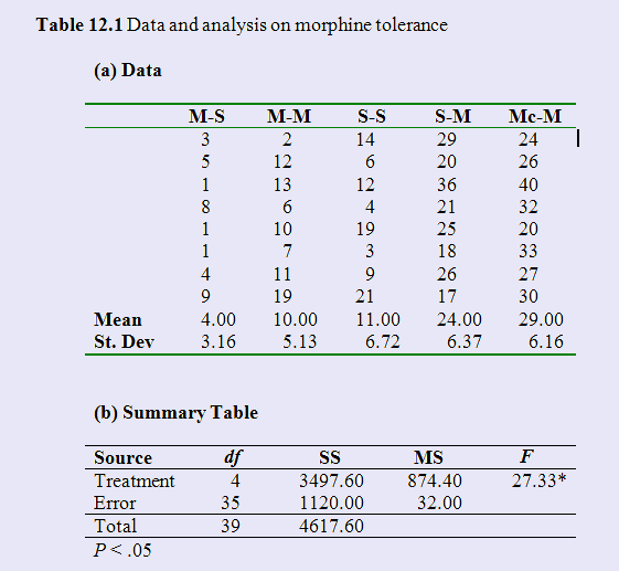
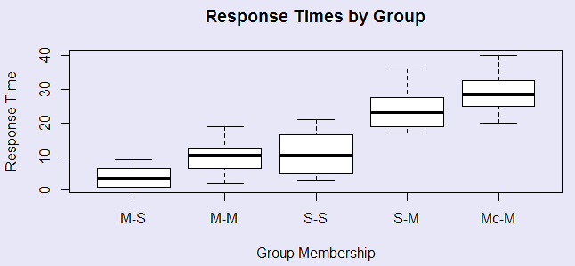
Siegel had five groups. Group M-S had morphine on three pretest trials and then saline on the test trial. It should be very sensitive to temperature. Group M-M had morphine on all trials, and because it has buiilt up a tolerance to morphine, it should be quite sensitive.It should be quite sensitive. Group S-S always had saline, so should be fairly sensitive. Group S-M had saline of the pretest trials and morphine on the test trial, and group Mc-M always had morphine, but the test trial was in a novel apparatus. These two groups should be the least sensitive to the temperature because they have morphine on the last trial to compensate. The data are shown below, along with the simple analysis of variance on these 5 groups. It is apparently that there are significant differences between the group means. We can see this most easily in the boxplot given in the figure. The two groups that received morphine in the testing environment for the first time on the test trial showed the longest latencies, and thus the least morphine tolerance.
To obtain this analysis in R, we simply read the data and call an analysis of variance function. However, when you look at the code, things appear to be a little odd. The first function that is called is lm(), which stands for "linear model." But because the independent variable is a factor, it is not what you think of as standard regression. Once we have our model ("model1"), the next function summary.aov displays the result as a standard analysis of variance table. The code is shown below, along with the result, which is set off with "#".
data <- read.table("Tab12-1.dat", header = T)
Group <- factor(data$Group, labels = c("M-S", "M-M", "S-S", "S-M", "Mc-M"))
Time <- data$Time
boxplot(Time ~ Group, main = "Response Times by Group", xlab = "Group Membership",
  ylab = "Response Time" )   # This was shown above.
model1 <- lm(Time ~ Group)
summary.aov(model1)
#                 Df Sum Sq Mean Sq F value   Pr(>F)
#     Group        4   3498   874.4   27.32 2.44e-10 ***
#     Residuals   35   1120    32.0
#     ---
#     Signif. codes:  0 ‘***’ 0.001 ‘**’ 0.01 ‘*’ 0.05 ‘.’ 0.1 ‘ ’ 1
Let me explain this procedure a bit. Notice that Group is a factor with 5 levels. This is the independent variable, and because it is a factor it is not something that we would likely use if we were focusing on a regression problem. Time is a continuous variable, which is common for dependent variables. Using "lm(Time ~ Group)" predicts the dependent variable (Time) as a function of the factor (Group). Because Group is a factor, R creates the appropriate group contrasts internally, and uses those in the regression.
It would be reasonable to think of "model1" as cobtaining the anova that you want. But if you print out model1, you get
Coefficients:
(Intercept)     GroupM-M     GroupS-S     GroupS-M    GroupMc-M
          4            6            7           20           25
which is not at all what you probably expected. What you really have here is a regression equation, telling you that the first group (M-S) had a mean of 4, that the second group differed from that by 6 points, the third group was 7 points above the base group, etc. That is nice, but it is not what you wanted. To get what you want, you need a summary of model1, and that summary should be in analysis of variance format. That is why I used "summary.aov(model1)" above.
As you can see, this analysis reproduced the analyses given above, with an F = 27.32. At one level, that is what we requested, and we can be satisfied. However, we might quite legitimately want a result that includes group contrasts in the output. We can get those contrasts, but they may not be quite what you expected. The reason for this is that R uses a default of treatment contrasts, which takes the first group as the base, and compares each group to that. So our result, when we use summary.lm(model1), is:
summary.lm(model1)
#     Coefficients:
#                 Estimate Std. Error t value Pr(>|t|)
#     (Intercept)    4.000      2.000   2.000   0.0533 .
#     GroupM-M       6.000      2.828   2.121   0.0411 *
#     GroupS-S       7.000      2.828   2.475   0.0183 *
#     GroupS-M      20.000      2.828   7.071 3.09e-08 ***
#     GroupMc-M     25.000      2.828   8.839 1.93e-10 ***
#     ---
#     Signif. codes:  0 ‘***’ 0.001 ‘**’ 0.01 ‘*’ 0.05 ‘.’ 0.1 ‘ ’ 1

#     Residual standard error: 5.657 on 35 degrees of freedom
#     Multiple R-squared:  0.7574,    Adjusted R-squared:  0.7297
#     F-statistic: 27.32 on 4 and 35 DF,  p-value: 2.443e-10
This result goes further than we had when we just asked for model1 to be printed out, and it includes the F value from the Anova.
Notice that for this result, the intercept is the mean of the first group (M-S), and the other estimates are deviations of each of the other group means from the mean of the first group. This is because we used treatment contrasts, which are the default in R. That does not strike me as a particularly useful set of contrasts. Perhaps I might feel better if I could make the S-S group the referent. At least it represents a clear control group. I can do that by specifying the base level as Group 3. This is shown below, where we see that all of the groups except Group M-M differ from that control group.
contrasts(Group) = 'contr.treatment'(levels(Group), base = 3)
model2 <- lm(Time ~ Group)
summary(model2)
summary.lm(model2)
#     Coefficients:
#                 Estimate Std. Error t value Pr(>|t|)
#     (Intercept)   11.000      2.000   5.500 3.52e-06 ***
#     GroupM-S      -7.000      2.828  -2.475   0.0183 *
#     GroupM-M      -1.000      2.828  -0.354   0.7258
#     GroupS-M      13.000      2.828   4.596 5.40e-05 ***
#     GroupMc-M     18.000      2.828   6.364 2.57e-07 ***
As I said, R uses contrasts called "treatment contrasts", denoted as "contr.treatment," by default. If we use what are called "sum contrasts" instead, our overall F will not be affected, but the coefficients will be in terms of the grand mean and deviations of group means from the grand mean. I won't show that here, but it is easy to do by simply changing to "contrasts(Group) = 'contr.sum'.
If you consider what you do in SPSS or SAS (a comparison that usually upsets true R devotees), you do some of the same things for some contrasts. For example, in SPSS you can have a statement that reads "/CONTRAST(Group)=Helmert", or "/CONTRAST(Group)=Simple", etc. Helmert contrasts compare the 1st group with the all subsequent levels, the 2rd with the average of the levels 3, 4, 5, etc., and so on. (R reverses the ordering of groups (1st with 2nd, 1st and 2nd with 3rd, etc.), "/CONTRAST(Group) = Simple" compares each group with a reference group. R allows basically the same thing. You can simply state " contrasts(Group) = contr.helmert" to get Helmert contrasts. Similar statements will give you other standard contrasts. So that part is easy. You just embed such statements in the following and get the result you seek.
contrasts(Group) <- contr.helmert
model1 <- lm(Time~Group)
summary(model1)
Perhaps I just work in the wrong field, or perhaps I am just a crab, but I find that whole set of possible contrasts, such as Helmert, to be less than helpful. In my experience, the ordering of treatments is often quite arbitrary, and I can't say that the second should be compared to the first or the third compared to the average of the first two. That might happen, but I haven't yet seen a case. The same applies to similar kinds of available contrasts. In my experience a set of five means might have two, three, or four useful specific contrasts, but I want to be able to specify what they are and not let the program do that for me or lock me in to a specific set.
Let us go one step further and specify a couple of contrasts in which we have particular interest. I am going to use contrasts that are orthogonal, because we run into some difficulties when we use nonorthogonal contrasts. For this example I will make four comparisons, using up my 4 df between groups. I want to compare the mean of the last two groups for which morphine would be expected to have maximum benefit on the test trial (S-M and Mc-M) with the first three groups. I also want to compare the group that first received morphine on the test trial with the group that received morphine in a new context. (S-M vs Mc-M). Finally I will compare M-M with S-S to see if four trials of morphine leave an animal in the same state he would be in without any morphine. At his point I am going to throw in a 4th comparison, in which I may not have any interest, just to use up my 4 df for Groups. I will explain why shortly. This will leave me with the following set of coefficients.
-1/3, -1/3, -1/3, 1/2, 1/2
0, 0, 0, 1, -1
0, 1, -1, 0, 0
2, -1, -1, 0, 0
I can set these contrasts to work by first creating a matrix of coefficients and then assigning that to group contrasts. However, I want to make sure that they print out in a way that they are easily read, so I add some code to the summary command, and use "summary.aov" in place of "summary.lm".
contrasts(Group) <- matrix(c(-1/3, -1/3, -1/3, 1/2, 1/2, 0, 0, 0, 1, -1, 0, 1,
   -1, 0, 0, 2, -1, -1, 0, 0), nrow = 5, ncol = 4)
summary.aov(model3, split=list(Group=list("First 3 vs S-S and Mc-M"=1, "S-M vs Mc-M" = 2,
 "M-M vs S-S"=3)))
#                                    Df Sum Sq Mean Sq F value   Pr(>F)
#  Group                             4   3498     874  27.325 2.44e-10 ***
#    Group: First 3 vs S-S and Mc-M  1   3168    3168  99.008 9.66e-12 ***
#    Group: S-M vs Mc-M              1    100     100   3.125   0.0858 .
#    Group: M-M vs S-S               1      4       4   0.125   0.7258
#    Residuals                      35   1120      32
---
Signif. codes:  0 ‘***’ 0.001 ‘**’ 0.01 ‘*’ 0.05 ‘.’ 0.1 ‘ ’ 1
Notice that Groups S-S and M-M do not differ, suggesting that tolerance develops very quickly. This set of contrasts makes a certain amount of logical sense, and I am happy with them. However, if the contrasts had not been orthogonal, for example if the third compared S-S with M-S, life would not be quite so simple. For example, most texts, my own included, use the word "contrast" in a different way from the way that the people who wrote R use it. To me, the "contrasts" are the weights (e.g. 1, -2, 1, 0, 0), whereas for R the contrasts are a coding scheme. If you take the coefficients as I would give them, R uses the inverse of that matrix of coefficients. It is fine when the contrasts are orthogonal, but not when they are not. For a more extensive discussion of this problem, a very good link can be found at ContrastsInRShafer.pdf. I believe that the author of that document is Joseph Shafer who was at Penn State when he wrotee it.
Along the lines of what I just said, notice that I didn't have it print out the last contrast, which was the comparison of M-S with M-M and S-S. I don't really care about that contrast, but I put it in to keep things simpler. (You will see this when I come to using an inverses of a matrix, which requires a square matrix.
There are a couple of choices. In SPSS, SAS, and R you can specify a set of orthogonal contrasts, as we just did with our example. That is certainly getting closer to my ideal. But if the contrasts are not orthogonal, things become messy in R. If they are not orthogonal, R will get a result, but it is not the result you thought that you were getting.
So what is the problem? Well in SPSS or SAS, the program takes your matrix and automatically adjusts it to be what you need. You don't see this happening, but it happens anyway. That's good. But R takes itself more literally. It uses the matrix you give it, but it doesn't make a necessary adjustment because you didn't tell it to and it only does what you tell it. Now this doesn't make any real difference if your contrasts are orthogonal, but it does if they aren't.
What SPSS really does is to take the matrix of contrasts that you give it, augments it temporaily, takes the inverse of that matrix, deaugments that (if that is a word) and works with that inverse. It just happens by magic. If the original matrix was orthogonal, the inverse version is just a scalar function of that and it won't make any difference to the outcome which matrix you work with. So you specify the code that I gave above and you will get the right answer. But if the matrix is not a set of orthogonal coefficients, especially if it is not square, working directly with that matrix will give you the wrong answers for some of the contrasts -- and won't give you an inverse if you have a non-square matrix. The contrasts, assuming "squaredom" will look just fine, leaving you to think that you got what you wanted. So what does R really want us to do? It wants us to get the inverse ourselves. (If we have a nice neat complete set of orthogonal contrasts, it doesn't matter if we work with the inverse or the original matrix itself.)
Let's start with a matrix of contrasts that are orthogonal. Suppose that we have the same five means that we used above, but we set up a different matrix of contrasts. We can do this as follows (or we could use the pattern above if you prefer).
L <- matrix(c(1/5, 1/5, 1/5, 1/5, 1/5,
 -1/3, -1/3, -1/3, 1/2, 1/2,
1, 1, -2, 0, 0,
1, -1, 0, 0, 0,
0, 0, 0, -1, 1), nrow = 5)
You may wonder about the first row of that matrix, but it sets up a column that represents the grand mean. (You could use 1,1,1,1,1 in place of the 1/5s if you prefer) It is there largely to make the matrix square so that we can take its inverse. We do that by
LInv <- solve(t(L))
myContrasts <- LInv[,2:5]
contrasts(Group) = myContrasts
So what is all that. The first command takes the inverse (R likes the word "solve") of the transposed augmented matrix. The next line removes the first column from that matrix--what I called "deaugmenting". The third line sets that new matrix up as the specified contrast matrix. This is what SPSS does behind the scenes where you don't see it. Now we are ready to find out what differences are significant. But we will do so with an actual example.
I give an example where the contrasts are not orthogonal. I compute the matrix of coefficients (L), take its inverse, drop the first column, and use that for my contrasts. You can try yourself using a slightly modified version of L instead of Linv as the contrast matrix, and see that the results are different (and wrong). The following code will produce the result we seek. The file can be found at onewayexample.r in a slightly different version.
###______________________________________________________
# The following gives correct solution for nonorthogonal design
# Notice that it uses the Linverse
# I need to use the Linverse with nonorthogonal designs
setwd ("C:\\Users\\Dave\\Dropbox\\Webs\\methods8\\DataFiles   ")
dat <- read.table("Tab12-1.dat", header = T)
Group <- factor(dat$Group)
Time <- dat$Time
#  I am specifying the contrast matrix as L and its inverse as LInv
L <- matrix(c(1,1,1,1,1,
-1/3, -1/3, -1/3, 1/2, 1/2,
1, 1, -2, 0, 0,
1, 0, 0, 0,-1,       # Not orthogonal to the above
0, 0, 0, -1, 1), nrow = 5)
Linv <- solve(t(L))
new.contrasts <- Linv[,2:5]
contrasts(Group) = new.contrasts
model4 <- lm(Time~Group)
summary.lm(model4,split=list(Group=list("First 3 vs last 2"=1, "First two vs third" = 2,
 "First vs Fifth"=3, "Fourth vs fifth" = 4)))

 #  The following (Using L instead of Linv)  will give the wrong answer
contrasts(Group) = L[,2:5]  # We need to get rid of that first row.
model5 <- lm(Time~Group)
summary.lm(model5,split=list(Group=list("First 3 vs last 2"=1, "First two vs third" = 2,
 "First vs Fifth"=3, "Fourth vs fifth" = 4)))
That's all there is to it. And don't think that you need four contrasts just because you have four df for Groups. Don't run things just because you can--run them because they ask relevant questions. The more tests you run, the more you increase the probability of a type I error. But I have found that it is safer to put in a full set of contrasts, but then to totally ignore the one that you don't care about. For one thing, that makes taking the inverse a lot easier.
dch:
David C. Howell
University of Vermont
David.Howell@uvm.edu