![]()
![]()
Assume that a large Fortune 500 company has set up a hotline as part of a policy to eliminate sexual harassment among their employees and to protect themselves from future suits.) This hotline receives an average of 3 calls per day that deal with sexual harassment. Obviously some days have more calls, and some have fewer. We want to model the distribution of calls over the course of an extended period of time. We will assume that there is no seasonal variation in the number of calls. This is a situation that is ideal for illustrating the Poisson distribution. (The word is capitalized because the distribution is named after a 19th century French mathematician named Simeon-Denis Poisson.)
Before I continue, let me point out something important about the problem as I have stated it. I said that the hotline receives 3 calls per day. I did not say was that 3 out of 20 calls concerned sexual harassment, or anything similar. In other words, I have told you how many calls were about sexual harassment, but have told you nothing about some other category of calls. This will become important when we compare this distribution to the binomial distribution.
The important parameter, in fact the only parameter, of the Poisson distribution is μ, which represents the mean of the distribution. In our case, μ = 3, because I have said that the average number of calls per day is 3.
The distribution that we seek would tell us the probability of 0, 1, 2, 3, ... calls per day. This probability is given by the Poisson distribution as
For example, the probability of 2 calls about harassment in a day can be calculated as
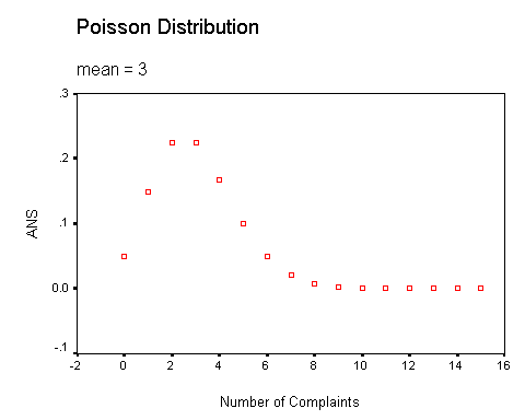
If we let x (the number of calls) take on all values between 0 and some arbitrarily high number, and if we substitute m = 3, we will obtain the following values for p:
x p 0
1
2
3
4
5
6
7
8
9
10
11
12
13
14
15.0498
.1494
.2240
.2240
.1680
.1008
.0504
.0216
.0081
.0027
.0008
.0002
.0001
.0000
.0000
.0000
In this example, once the values of x exceed about 10, the probabilities are so low that there is little point in calculating them. This distribution is plotted below.
We already know that the mean of the Poisson distribution is m. This also happens to be the variance of the Poisson. Thus we can characterize the distribution as P(m,m) = P(3,3).
An important feature of the Poisson distribution is that the variance increases as the mean increases. In many situations this makes considerable sense. If the mean for harassment calls is 3, we can reasonably expect the daily frequencies to fall between about 0 and 6. On the other hand, if the mean were 20, we would probably expect the daily frequencies might fall anywhere between 12 and 30. Obviously the variance will be larger in the second case.
You are probably most familiar with the normal distribution, because it underlies most of the standard statistical procedures that we use. For the normal distribution the mean and variance are independent, and there we would not expect the variance to increase as the mean does.
An important, though unfortunate, feature of many samples of data is that the variability of the results is greater than would be predicted by the Poisson distribution. The example used here is probably a good example of what can go wrong. You should recall that I assumed at the beginning that day to day observations of the number of calls are independent of one another. Thus, for example, the fact that we had 5 calls today should not be relevant in predicting the number of calls we will receive tomorrow.
However, if we are dealing with sexual harassment, I would think it likely that observations are not truly independent. There is probably some seasonable variation in harassing behaviors. It seems reasonable, for example, that women would receive fewer obnoxious remarks when they wear bulky sweaters in the winter than they would when they wear lighter clothing in the summer. If this were the case, the variability of the daily frequencies would reflect not only the natural variability we expect with a Poisson distribution, but also variability due to seasonal causes. Thus the actual variance is likely to exceed m.
The result of having overdispersion is that the Poisson distribution may not completely model the data at hand. There really is very little that we can do about this, unless we can find a model for the increased variance, but it is important to recognize. We find that the Poisson is a very nice model for many kinds of data, but don't expect that it will model everything.
The reason why I have discussed the Poisson distribution is that it is frequently a useful way of modeling categorical data. This is particularly important when the overall sample size (N) is not fixed, but is treated as a random variable. We can model each category count as a Poisson variable, and derive our hypothesis tests, and confidence intervals, on the basis of that model. Thus we might take each of the four cell counts in a 2X2 contingency table as an independent Poisson variable.
According to http://www.Tourettesyndrome.net/Tourette.htm, 3% of children in general education classrooms suffer from Tourette's syndrome, which is a disorder characterized by motor or verbal tics and possibly other disorders, including obsessions, impulsivity, compulsions, and disorders of mood. (I am not in a position to judge the accuracy of this 3% statistic, but will take it on faith.) Given this statistic, we might be interested in asking about the probability that an elementary school teacher will have at least one child in his classroom who suffers from Tourette's syndrome.
Notice that this problem is a bit different from the one we discussed with the Poisson distribution. In that situation I new the mean number of complaints per day of sexual harassment, and was interested in asking about the probability of receiving no calls today (or any other value that I might wish). But when I am faced with the example of Tourette's syndrome, it is logical for me to ask about the size of the class. For instance, I could ask "Out of a class of 20 students, how likely is it that one student will suffer from Tourette's syndrome?" Obviously, if the teacher has more students, he is more likely to have at least one with Tourette's syndrome.
For this situation I am going to fall back on the binomial distribution. This is a distribution that asks about the probability of x events out of N events. In other words, it allows me to ask about the probability of 1(or 2, or 3, etc.) Tourette's child out of a class of 20.
The formula for the binomial is given as
where N = the size of the sample, p = the probability of a successful outcome, q = 1 - p, and x = the number of "successes" in question.
Suppose that the teacher has 20 children in his class and he wants to know that probability that 1 of them will be a Tourette's child. Then N = 20, p = .03, q = .97, and x = 1. The probability can be obtained as
Thus the probability is .34 that the teacher will have exactly one child in his classroom with Tourette's syndrome.
Perhaps our teacher is more interested in knowing the probability that none of this children would have Tourette's syndrome. The arithmetic is even easier here, and the result is
For completeness, you could calculate that p(2) = .0988, p(3) = .0183, and p(x>4)=.0027.
The mean of the binomial distribution is always equal to p, and the variance is always equal to pq/N. Moreover, for reasonable sample sizes and for values of p between about .20 and .80, the distribution is roughly normally distributed.
Mean = p; Variance = pq/N; St. Dev. =
It is important to realize that the mean and variance above are given for the case where we are dealing with proportions. In other words, if we calculated the proportion of children in each of many classrooms who were suffering from Tourette's syndrome, the mean proportion would be p, and the variance of the proportions would be pq/N. However, if we want to speak, as we did above, about the number of children in the classroom who suffered from Tourette's syndrome, the mean number would be Np and the variance of the number of children across classrooms would be Npq. It is important to keep in mind whether you are talking about proportions or frequencies. You can do it either way, as long as you are consistent.
Knowing that the binomial distribution is approximately normal for reasonable N and for .20 < p < .80, we can calculate the necessary cumulative probabilities by solving
And finding the lower-tailed probability of z from tables of the normal distribution. The probability obtained in this way will approach the probability obtained from direct calculations as the sample size increases.
An essential feature of the binomial distribution is the overall sample size. Thus we ask about the probability of x successes out of N trials. The binomial will therefore be useful when we can treat the same size as fixed. Thus, for example, if we took 50 men and 50 women and asked whether they had been the recipient of what they would class as acts of sexual harassment, we could model the number of each group, out of 50, who report harassment.
When we were speaking of the Poisson distribution, we did not know how many calls there would be each day. In this case, N was a random variable. This is an important characteristic of the Poisson distribution.
Suppose, however, that we modified our design to wait for 20 calls, of various kinds, to come in each day, and tallied the number of calls, out of 20, that related to sexual harassment. Here the sample size (20) is fixed, rather than random, and the Poisson distribution does not apply.
The sampling plan that lies behind data collection can take on many different characteristics and affect the optimal model for the data. The way in which we model data may affect the analysis we use.
With the Poisson distribution, we know the mean (m), but not the sample size. Suppose, to extend the example of sexual harassment, we sort the calls we receive into allegations of sexual harassment and allegations of other misbehaviors. We also sort the calls into those alleging infractions by co-workers and those alleging infractions by superiors. Because the total sample size is a random, not a fixed, variable, we could model the data by treating each of the four cell counts as independent Poisson variates.
Often we have a fixed total sample size, but the row and column totals are random. For example, we might sample 200 respondents (a fixed number) and sort them by both gender and attitude toward abortion (opposed, not opposed). Here we could treat the data as a multinomial distribution with four categories. (The multinomial distribution is the extension of the binomial distribution to the case of more than 2 categories.) This is a legitimate way to treat the data, but when one dimension of the table (e.g. rows) is treated as an explanatory variable, and the other as a response variable, it often makes the most sense to treat the row totals as if they were fixed, and to compare the conditional distributions within each row.
Often the row variable in a contingency table will refer to a grouping variable, and we know what the row totals will be. For example, we might assign 150 patients to one treatment and another 150 patients to another treatment, and categorize the resulting outcomes as "improved" and "not improved." Here we know the row totals and can treat them as fixed. The column totals are unknown, until the data are collected, and we treat them as random. Here we can model our results with a separate binomial distribution for each row, with the sample size fixed as equal to the row total.
In the preceding paragraphs we have considered different ways of modeling the data. Fortunately, we don't have to worry overmuch about which model is most appropriate (Poisson, binomial, or multinomial) because the different models lead to the same results in our analysis. Why then, you might ask, did I muddy the waters by this digression? The answer is that most texts in this field make the distinctions that I have, even if they then claim that the same results apply across models. I am trying to help myself understand how the models differ, and I hope that I am helping you as well. If you are still suffering from some level of "yes, but ...," you are not alone.
![]()
![]()
 Return to Dave Howell's Statistical Home
Page
Return to Dave Howell's Statistical Home
Page
 University of Vermont Home Page
Last revised 1/3/2003