

This web page is a step by step demonstration of using NORM (http://sites.stat.psu.edu/~jls/misoftwa.html) to handle multiple imputation. It is deliberately not a theoretical discussion. The first draft was a big mess, and I hope that this draft is just a little mess.
The data file is named Cancer.dat and contains the following variables related to child behavior problems among kids who have a parent with cancer. Most of the variables in this example (a truncated data set) relate to the parent (patient) with cancer. The variable names are, in order, SexP (sex parent), deptp (parent's depression T score), anxtp (parent's anxiety T score), gsitp (parent's global symptom index T score), depts, anxts, gsits (same variables for spouse), sexchild, totbpt (total behavior problem T score for child). These are a subset of a larger dataset, and the analysis itself has no particular meaning. I just needed a bunch of data and I grabbed some variables. We will assume that I want to predict the child's behavior problem T score as a function of the patient variables. I no longer recall whether the missing values were actually missing or whether I deleted a bunch of values to create an example.
The first few cases are shown below. Notice that variable names are NOT included in the first line. Missing data are indicated by -9. NORM only allows a few codes for missing, and -9 is one of them, but "." is not. (If you are using the norm library in R, you need to replace the "-9" by "NA".)
2   50   52   52   44   41   42   -9   -9
1   65   55   57   73   68   71   1   60
1   57   67   61   67   63   65   2   45
2   61   64   57   60   59   62   1   48
2   61   52   57   44   50   50   1   58
1   53   55   53   70   70   69   -9   -9
2   64   59   60   -9   -9   -9   -9   -9
1   53   50   50   42   38   33   2   52
2   42   38   39   44   41   45   -9   -9
2   61   61   55   44   50   42   1   51
1   44   50   42   42   38   43   -9   -9
2   57   55   51   44   41   35   -9   -9
-9   -9   -9   -9   57   52   57   2   65
2   70   59   66   -9   -9   -9   1   61
2   57   61   52   53   59   53   2   49
To enter the data start NORM.exe and select File/New Session. Then select the file, which I called CancerNorm.
The Help files are excellent (mostly), and I recommend that you read them carefully.
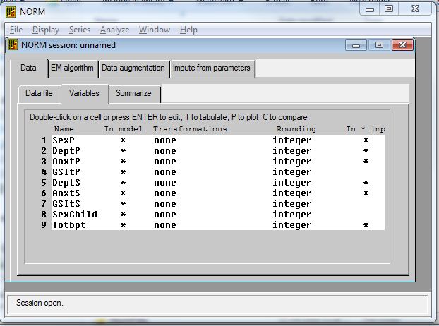
The NORM dialog box, assuming you click in the right place, looks like this--at least it will after you make changes.
When you click on the Variables button it allows you to enter names. Just double click on "Variable 1", or whatever it is called, and type in SexP. The same for all. But you have variables there that you do not want to use in the imputation, so find the * to the right of GSItP, GSItS, and SexChild and double click on those. They will go away.
If you want descriptive statistics, click on the Summarize button. Now you are ready to begin.
The first step that you want to carry out is to run the EM algorith. This estimates means, variances, and covariances in the data. First a bit of theory. EM looks at the data and comes up with estimates of means, variances, and covariances. Then it uses those values to estimate missing values. But when we add in those missing values, we come up with new estimates of means, variances, and covariances. So we again estimate missing values based on those estimates.
This, in turn, changes our data and thus our next estimates. But for a reasonably sized sample, this process will eventually converge on a stable set of estimates. We stop at that point.
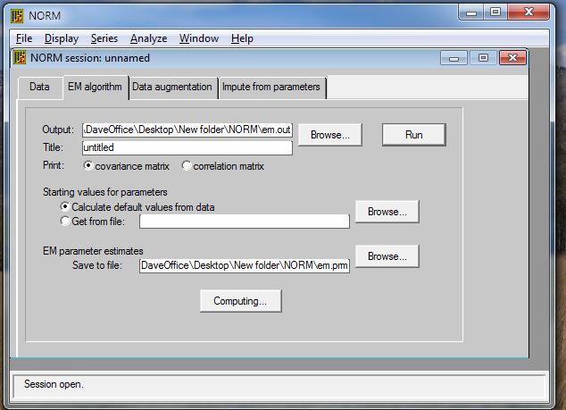
We run EM first before we go on to Data augmentation to get a reasonable set of parameter estimates. We don't have to do this first, but it speeds the process. You simply select the EM algorithm tab, give the output file a name (the default is em.out) You can specify the maximum number of iterations. If it does not converge by then, it will quit. The default is 1000. The parameter estimates that result from the EM algorithm are stored, by default, in a file named em.prm. I won't change this because then I would have to make the same change in subsequent steps that use this file. It's easier to go along with the defaults. Just click Run The results will appear. There are actually two files--one is for you to read and the other (em.prm) is for NORM to use later.
Next you want Data Augmentation. Data Augmentation (DA) is the process that does most of the work for you. It takes estimates of population means, variances, and covariances, either by taking the output of EM or by recreating them itself. Again we need a tiny bit of theory. Using the means, variances, and covariances, DA first estimates missing data. But then it uses a Baysian approach to create a likely distribution of the parameter values. For example, if bi with the adjusted data comes out to be 1.56, it is reasonable to expect that the population regression coefficient falls somewhere around 1.56 with a standard error approximately equal to the standard error of bi. But instead of declaring it to be 1.56, DA draws an estimate at random from the likely distribution of bi. This is a Baysian estimate because we essentially ask what would the distribution of possible coefficients really look like given the obtained sample coefficient. To oversimplify, think of calculating a bi on the basis of data. Then think of creating a confidence limit on the population parameter given that sample estimate. Suppose that the CI is 1.2 - 1.92. Then think of randomly drawing an estimate of βi from the interval 1.2 - 1.92, and then continuing with an iterative process. This is greatly oversimplified, but it does contain the basic idea. And, remember, we are going to continue this process until it converges.
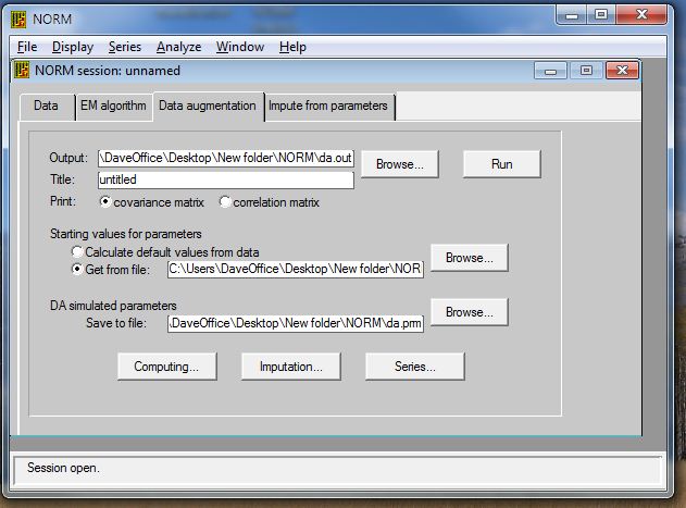
To run DA, you could take the defaults by clicking on the Data Augmentation tab. However, we need to do a little more because we want to create several possible sets of data. In other words, we want to run DA and generate a set of data. Then we want to run DA over again and create another set. In all we might create 5 sets of data, each of which is a reasonable sample of complete data with missing values replaced by estimated values.
Rather than run the whole program 5 times, what we do is to run it, for example, through 1000 iterations. In other words, we will go through the process 1000 times, each time estimating data, then estimating parameters, then re-estimating data, etc. But after we have done it 200 times, we will write out that data set and then keep going. After 400 iterations we will write out another data set, and keep going. After the 1000th iteration we will write out the 5th data set. BUT don't do as I just did and type in 200 without clicking on the little button. Otherwise it won't write out any imputations. If you do it right you will see the files named Cancer_1.imp, etc. There should be 5. Even though these have funny extensions, they are really just txt or dat files. You can read them with any text editor.
Now you have 5 complete sets of data, each of which is a pretty good guess at what the complete data would look like if we had it. We would HOPE that whichever data set we used we would come to roughly the same statistical conclusions. For example, if our analysis were multiple regression, we would hope, and expect, that each set would give us pretty much the same regression equation. And if that is true, it is probably reasonable to guess that the average of those five regression equations would be even better. For example, we would average the five estimates of the intercepts, the five estimates of b1, etc. We won't do exactly this, but it is close.
But you might ask why I chose 1000, 200, and 5. Well, the 5 replications was chosen because Rubin (1987) said that 3 - 5 seemed like a nice number. Well, it was a bit more sophisticated than that, but I'm not going there. So let m = 5. But how many interations before we print out the first set of imputed data? Schafer and Olsen (1989) suggest that a good starting point is a number larger than the number of iterations that EM took to converge, which, for our data, was 56. So I could have used 60, but k = 200 seemed nice. Actually it was overkill, but that won't hurt anything, and you are not going to fall asleep waiting for the process to go on for k*m = 1000 times. It will take a couple of seconds.
This is the point at which we put NORM aside for the moment and pull out SPSS or something similar. We simply take our m = 5 datasets, read them each into SPSS, run our 5 multiple regressions, record the necessary information, and turn off SPSS. In fact, it would be much nicer if you wanted to use SAS because you can tell NORM to save the 5 sets of coefficients, along with the corresponding covariances, and then have SAS put them altogether. I'll write up a similar, but much shorter, document about SAS later. Much later.
I suggested above that you are basically just going to average the coefficients from the 5 regressions--or similar stuff from 5 analyses of variance, logistic regressions, chi-square contingency table analyses, or whatever. Well, that is sort of true. In fact for the actual coefficients that is exactly true. But we also want to take variability into account. Whenever you run a single multiple regression you know that you have a standard error associated with each bi. Square that to get a variance. But you also know that from one of the 5 analyses to another you are also going to have variability. We want to combine the within-analysis variance and the between-analysis variance and use that to test the significance of our mean coefficient. It took a while but I finally got NORM to do this for me. The nice thing about SAS is that I know how to set up the whole thing. But what follows is the hand solution taken from Schafer & Olsen (1998).
The following table is one that I created on the basis of 5 runs of multiple regression. The labels on the first line don't belong there, so if you create such a table, leave them out. Notice that the first line is the regression equation for the first imputed data set. The second line contains the standard errors of each of those coefficients. The 3rd line contains the equation for the 2nd set, followed by a line with the corresponding standard errors. This repeats for 5 data sets.
   b0       b1      b2      b3      b4      b5
-15.998  -1.8839  0.7239  0.1716 -0.2663  0.6407
  6.0860  1.5776  0.0831  0.0872  0.0899  0.0906
  0.6173 -4.8492  0.7490 -0.0600 -0.3926  0.7483
  6.6361  1.7340  0.0913  0.0989  0.1027  0.0934
  2.9619 -5.1756  0.6475  0.1427 -0.3717  0.6382
  6.5299  1.8161  0.1101  0.1042  0.1047  0.1067
-19.1318 -1.0913  0.7836  0.1687 -0.3944  0.7037
  6.8107  1.9266  0.1062  0.1026  0.1011  0.0942
-11.5540 -0.2896  0.8300 -0.1057 -0.5415  0.8412
  6.0248  1.6967  0.0954  0.0886  0.0914  0.0936
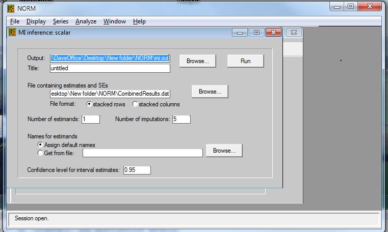
You need to create a file just like this. Name it whatever you want--eg., "CombinedResults.dat." Then go to the top menu of NORM and click on Analyze/MI Inference: Scalar. You will get the following.
You need to browse to find CombinedResults.dat and give the output file a name if it needs one. Don't stop yet. Go to the middle of that box and make the number of estimands equal to the number of variables plus the intercept. For my example that is 6. Also make sure that it knows that there are 5 imputations. Then click Run. There is a bug in this program somewhere. When I did it I was told that there were 10 nonblank lines but it needed 10. Strange. I finally got it to run by canceling that run and starting again. You might have to get out of NORM entirely and then get back in. This has happened more than once. You will see the output on the screen and should find a file named CombinedOutput someplace. It showed up in my NormProgram file, but I guess I was careless.
Now you are done. SAS is easier.
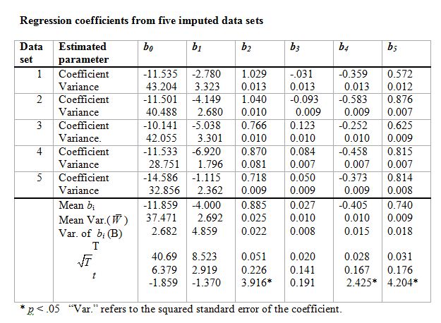
The following will not be needed if the last step works out. If you can't get it to run, read the following. I just left it in for that purpose. The table that follows contains the results of 5 imputations with the cancer data.
Thus the regression equation for the first set of data would be
Y = -11.535 -2.783*b1 + 1.029*b2 -0.031*b3 -0.359*b4 +0.572*b5.
The standard error of b1, for example, was 1.823, so its square (the variance) is 3.323, which you see in the table.
Notice that I have taken the means of the five bi. I have also taken the mean of the within imputation variances. Then I took the variance of the bi, shown in the third line at the bottom. Now I need to combine these two variances. This is calculated as
T = mean variance within (W) + (1 + 1/m)*variance (B) of the bi.
For b1 this is 2.692 + (1+1/5)*4.859 = 8.523.
The square root of this is 2.919, which is our estimate of the standard error of the estimated b1 = -4.000. If we divide -4.000 by 2.919 we get -1.370, which is a t statistic on that coefficient. So that variable does not contribute significantly to the regression.
You will note that I used multiple regression here. If I had used an analysis of variance on these data I would have run 5 Anovas and done similar averaging. I haven't really thought through what that would come out to, but it shouldn't be too difficult. I suspect that I would average the MSbetween, average the MSwithin, take the variance of the SSbetween, and combine as I did above.

 Return to
Dave Howell's Statistical Home Page
Return to
Dave Howell's Statistical Home Page
Last revised 11/19/2009