

It is often said that those with a strong religious faith have a more sanguine view of the world, perhaps because they see life in a broader context. Indeed, Marx is quoted often as saying that "Religion is the opiate of the people." Those with more liberal views of religion may take to themselves a greater responsibility for the conduct of their own lives, whereas the more fundamentalists sects or religions encourage their followers to accept a hierarchical structure in which unquestioning faith is expected of all. Such unquestioning faith might be expected to lead to less concern with the cares of the world, which in turn might lead to a greater optimism (or less pessimism) about the world and one's place in it.
Sethi and Seligman (1993) reported a study in which they looked at the relationship between optimism and religious fundamentalism. They were concerned with two broad issues. The first was whether religious groups differing in degree of fundamentalism varied in their level of optimism. The second was whether optimism could be predicted on the basis of several variables measuring the role of religion is the person's life.
Sethi and Seligman collected data from over 600 adults from nine religious groups. These nine groups were sorted into three major categories (Fundamentalists, Moderates, and Liberals) and those three categories formed the basis of future analyses.
The data that Sethi and Seligman collected were a measure of Optimism and three measures of the role of religion in the person's life--hereafter termed Religiosity. The Optimism measure was calculated from the Attributional Style Questionnaire. This scale can be seen at https://www.scribd.com/doc/188891410/Attributional-Style-Questionnaire-doc and measures causal explanations for both positive and negative events along three dimensions: Stability-Instability, Internality- Externality, and Global-Specific. The data involve a combined score across these three dimensions for both the positive and negative items, and the difference between the positive and negative scores was taken as the subject's optimism score.
Sethi and Seligman also used a questionnaire designed to measure Religiosity. They assessed the influence of religion in daily life (RInfluen) [e.g.,"To what extend do your religious views influence who you associate with?"], religious involvement (RInvolve) [e.g.,"How often do you attend religious services?"], and religious hope (RHope) [e.g.,"Do you believe there is a heaven?"] Each of these items was rated on a 7 point Likert scale (where 7 = agree) and the mean across the items on each scale was used as the dependent variable.
This study included other variables which are not relevant to this particular example. A critique of the specific methodology of this study can be found in Kroll (1994).
The data in this example were generated to match the data of Sethi and Seligman using a program written by Aguinis (1994). Many of the relevant statistics were given in the Sethi and Seligman paper, and those that were not given were estimated based on what seemed to be reasonable values for the variables involved. The fact that the results largely agree with those given by Sethi and Seligman testifies both to the fact that the estimates were reasonable and that with large sample sizes effects are sufficiently robust to overcome any differences in the estimates.
The data were generated by first using Aguinis's program to generate 600 cases sampled from a population with a specified pattern of correlations. Since these data were samples from a population, there was no guarantee that the sample correlations would be exactly as specified, so repeated samples were taken until the pattern of correlations was satisfactory.
Once the data were generated, they were read by a SAS program which assigned them to three groups simply on the basis of desired sample size the first 200 cases were assigned to the Fundamentalist category, the next 280 were assigned to the Moderate category, and the final 120 were assigned to the Liberal category. (The unequal sample sizes were a near approximation of the samples obtained by Sethi and Seligman.) The data were first standardized to a mean of 0 and a standard deviation of 1 for each group separately, and then transformed to have means and standard deviations matching those of Sethi and Seligman. This matching is easily accomplished because if you start with data with mean = 0 and std = 1, you can produce any mean and standard deviation you desire by
Newdata(i) = St. dev*Olddata(i) + Mean
The data were then rounded to integers to make them more realistic. The rounding affected the means and standard deviations only slightly, and had only a minor effect on the pattern of correlations. Again, the large sample sizes helped. It is important to keep in mind that a linear transformation of data changes the means and standard deviations, but does not alter the correlation between variables. Therefore once the data are produced to have a specific pattern of correlations, further transformations leave those unaffected.
The data that were generated can be found at Fundamentalism.dat in text form. The variables, in order, are
The analyses for this example fall in two parts. The first asks whether the three religious categories differ in Optimism. The second tries to explain Optimism in terms of variables associated with Religiosity. In addition, the second set of analyses asks whether differences in Optimism between the categories remain after we take religiosity into account.
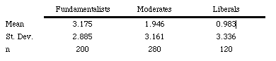
The means and standard deviations of the three religious groups are given below. From these means it is clear that Fundamentalists exhibit a higher level of Optimism than do Moderates, who, in turn are more optimistic that liberals.
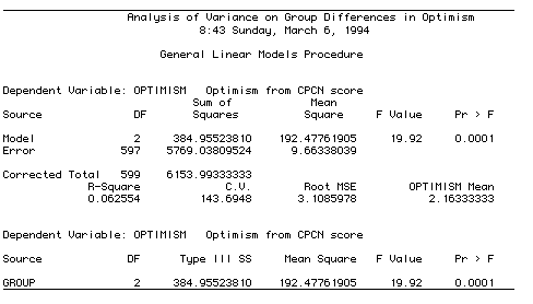
The analysis of variance comparing the three religious groups reveals a significant main effect for Groups (F(2,597) = 19.92, p = .0001).

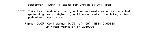
I chose to run Bonferroni tests among the three group means to illustrate the result. All differences are significant. These analyses are shown below. A Newman-Keuls test would also have been appropriate, and would also hold the maximum familywise error rate at differences.
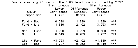
The Bonferroni printout is somewhat different from what we obtain with range tests such as the Newman-Keuls and Tukey. For each pairwise comparison, e.g., Fund vs Mod, we see the actual difference between the means (1.229), and confidence limits on that difference (0.539-1.920). Because this confidence interval does not include 0.00, the difference between means is significant, and this is indicated by "***" in the right-hand column. Notice that the pattern of differences tells us that Fundamentalists are more optimistic that Moderates, who are in turn more optimistic that Liberals.
These results support the hypothesis that greater religious fundamentalism is associated with a more optimistic view of life. The fact that the standard deviations of Optimism scores were quite similar for all three groups reveals that there is a similar degree of diversity within each level of Fundamentalism, which is itself an interesting result.
rm(list = ls())
### Analysis of Fundamentalism data from Sethi and Seligman

setwd("~/Dropbox/StatPages/Fundamentalism")
data <- read.table("Fundamentalism.dat", header = TRUE)
attach(data)
options(digits = 5)
Group <- factor(Group)
tapply(Optim, Group, mean)
tapply(Optim, Group, sd)
model1 <- lm(Optim ~ Group)
print(anova(model1), digits = 5)
library(asbio)   # To run Bonferroni correction
pairw.anova(Optim, Group, method = "bonf")
__________________________________________________________

Analysis of Variance Table

Response: Optim
           Df Sum Sq Mean Sq F value    Pr(>F)
Group       2    385 192.478  19.918 4.227e-09 ***
Residuals 597   5769   9.663
---
> pairw.anova(Optim, Group, method = "bonf")

95% Bonferroni confidence intervals

                Diff    Lower    Upper  Decision Adj. p-value
muFund-muLib 2.19167  1.32992  3.05341 Reject H0            0
muFund-muMod 1.22857  0.53764  1.91951 Reject H0      6.9e-05
muLib-muMod  -0.9631 -1.77737 -0.14882 Reject H0     0.014016
> contrasts
The fact that the three religious categories differ in their level of optimism does not tell us why. It is possible, as suggested in the introduction, that the structure of those religious traditions, with more or less emphasis on hierarchical organization and dogma, is the controlling variable. It is also possible that the religious practices and attitudes, such as religious influence, involvement, and hope, can explain the pattern.
One preliminary analysis that should be included in a complete analysis, but which will be omitted here simply because an example such as this cannot afford to try to do everything at once, would look at group differences in religious influence, involvement, and hope. If such differences do exist, and it is likely that they do, then any analysis is plagued with the problem of confounding the categories of fundamentalism and Religiosity. I leave that concern as something that you should think about, and the data are available in the data file.
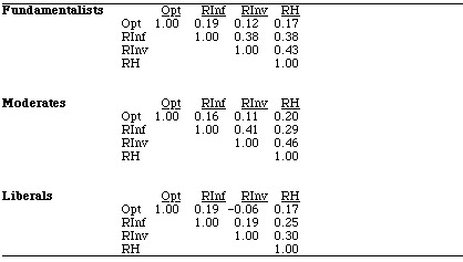
The first analysis looks at the intercorrelations among the variables. The following tables show the intercorrelations for the three separate religious categories. To save space I have abbreviated the variable names.
rm(list = ls())
### Analysis of Fundamentalism data from Sethi and Seligman

# Assumes that the above code has already been run.

data <- data[,-1]      # Remove ID as variable
tempdata <- (subset(data, data$Group == 1))
tempdata <- as.matrix(sapply(tempdata, as.numeric))   # converts dataframe to matrix
cor(tempdata)
tempdata <- (subset(data, data$Group == 2))
tempdata <- as.matrix(sapply(tempdata, as.numeric))   # converts dataframe to matrix
cor(tempdata)
tempdata <- (subset(data, data$Group == 3))
tempdata <- as.matrix(sapply(tempdata, as.numeric))   # converts dataframe to matrix
cor(tempdata)
Although the pattern of correlations is almost identical across the three matrices, the best way to combine the data is to calculate what is called a Within-Groups correlation matrix. This is obtained by taking a weighted average of the three matrices, where the weights are the degrees of freedom, and where we average the Fisher-transformed values of r and then perform a back- transform on the results. The purpose of computing separate matrices and averaging, rather than tossing all 600 subjects in together and calculating the matrix, is that the within-groups matrix eliminates any influence of group differences.
As an example, the average correlation of Religious Involvement with Religious Hope is
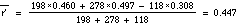
The back-transform of this value of r' is 0.42. Similar calculations on the other cells produces

Each of these correlations is significant at p < .05, as can be shown with a t test on 594 df, and most are significant at p ‹ .001. Here you can see that the religiosity variables are correlated more highly with themselves than with the Optimism variable. This is not surprising, and, to be honest, these are values that I generated because the published report did not give them. They seem reasonable to me. Notice also that each of the religiosity variables is itself correlated with the Optimism score (Those correlations are approximations of those given by Sethi and Seligman .)
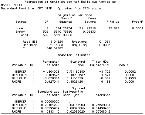
The next step in the analysis is to regress Optimism on the 3 religiosity variables. The SAS commands for this analysis follow, and are in turn followed by the analysis itself.
***** Regression of Optimism on RInfluen, RInvolve, and RHope;

### Assumes that previous analyses are already run.
> model2 <- lm(Optim ~ RelInf + RelInv + RelHope, data = data)
> summary(model2)

Call:
lm(formula = Optim ~ RelInf + RelInv + RelHope, data = data)

Residuals:
    Min      1Q  Median      3Q     Max
-12.720  -2.132   0.179   1.904   8.928

Coefficients:
            Estimate Std. Error t value Pr(>|t|)
(Intercept)  -1.8949     0.5118   -3.70  0.00023 ***
RelInf        0.4896     0.1071    4.57  5.9e-06 ***
RelInv       -0.0794     0.1163   -0.68  0.49529
RelHope       0.4279     0.1023    4.18  3.3e-05 ***
---
Signif. codes:  0 ‘***’ 0.001 ‘**’ 0.01 ‘*’ 0.05 ‘.’ 0.1 ‘ ’ 1

Residual standard error: 3.04 on 596 degrees of freedom
Multiple R-squared:  0.103,	Adjusted R-squared:  0.0985
F-statistic: 22.8 on 3 and 596 DF,  p-value: 5.32e-14
In this analysis, the F for the model is 22.828, which is significant at p = .0001. Thus we see that three religiosity variables taken as a set predict Optimism at better than chance levels. However we already knew that this would be the case because each of those variables predicted Optimism on their own. From this analysis we can see that the Multiple correlation squared is 0.1031, which gives a multiple correlation of 0.32, which is considerably higher than each of the individual correlations (the largest of which was 0.185.)
If we look at the tests on the parameter estimates we see that RInfluen and RHope contribute significantly to the result, but that RInvolve does not. Sethi and Seligman found a similar pattern of significance for these predictors.
The tolerance values for all three predictors reveal only modest overlap among the three measures of religiosity. For example, the tolerance for RInfluen is 0.755, meaning that the squared correlation of RInfluen with RInvolve and RHope is 1 - 0.755 = 0.245. Taking the square root we obtain a multiple R of .49, which, while large, is not nearly large enough to cause a problem with multicollinearity. The other tolerances are of generally the same magnitude.
The optimal regression equation given this set of predictors is
Optim = 0.490*RInfluen + 0.079*RInvolve + 0.428*RHope + 1.895
Even though RInvolve was a significant predictor of Optimism when taken alone, the very small t for RInvolve in the multiple regression suggests that we might be better off dropping that predictor and recalculating the regression The squared semi- partial for RInvolve is only 0.0007, where makes it clear that this variable adds virtually nothing to the regression over and above what the other two predictors contribute. I won't take the space to do that here, but a complete analysis would involve that step.
These results show that differences in people's level of Optimism can be directly related to a global variable of Religiosity. In particular, those who report that religion has a great influence on their life and who hold to views characterized as "religious hope" involving heaven and future reward for suffering show a greater level of optimism. Interesting, religious involvement, measuring such things as prayers and attendance at religious services did not explain optimism. This is in part a function of the fact that this variable overlaps with the other two predictors. But even taken alone, its correlation with Optimism was quite low (r = 0.08).
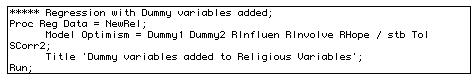
I earlier raised the problem that if the religiosity variables are themselves related to the three different levels of fundamentalism, then Religiosity and Fundamentalism are confounded. The three groups may differ in optimism because they differ in the structural aspects of their religion, or because they differ in what I have called religiosity, or some combination of both. It is a characteristic of non-experimental research such as this that such questions cannot be answered unequivocally. There is, however, a way to get a handle on the contribution of Fundamentalism over and above Religiosity. This is accomplished by adding predictors associated with the different levels of Fundamentalism to the equation after having considered Religiosity.
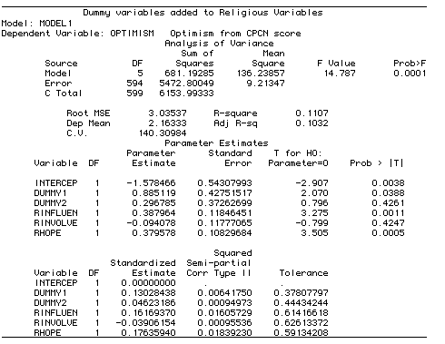
To regress optimism on fundamentalism, I need to create two dummy variables that code for group differences in fundamentalism. These variables are created in the appended SAS program. The first variable (Dummy1) is coded as 1 if the subject is in the Fundamentalist group, and 0 otherwise. The second dummy variable (Dummy2) is coded 1 if the subject is in the Moderate group and 0 otherwise. Subjects in the Liberal group have 0 on both dummy variables. These two variables are then treated as a set, and they are added to, or removed from, the equation together.
The regression with these two variables added to the other predictor variables follows:
### Assumes that previous analyses are already run.

### Adding the two dummy variables
dummy1 <- numeric(); dummy2 <- numeric()
dummy1 <- 0; dummy2 <- 0
for ( i in 1:600) {
   if (data$Group[i] == 1) dummy1[i] = 1
else(dummy1[i] = 0)}

for ( i in 1:600) {
   if (data$Group[i] == 2) dummy2[i] = 1
   else(dummy2[i] = 0)}

model3 <- lm(Optim ~ dummy1 + dummy2 + RelInf + RelInv + RelHope, data = data)
summary(model3)
_____________________________________________________________

Call:
lm(formula = Optim ~ dummy1 + dummy2 + RelInf + RelInv + RelHope,
    data = data)

Residuals:
    Min      1Q  Median      3Q     Max
-12.760  -2.169   0.173   2.021   8.661

Coefficients:
            Estimate Std. Error t value Pr(>|t|)
(Intercept)  -1.5785     0.5431   -2.91  0.00379 **
dummy1        0.8851     0.4275    2.07  0.03885 *
dummy2        0.2968     0.3726    0.80  0.42608
RelInf        0.3880     0.1185    3.27  0.00112 **
RelInv       -0.0941     0.1178   -0.80  0.42471
RelHope       0.3796     0.1083    3.50  0.00049 ***
---
Signif. codes:  0 ‘***’ 0.001 ‘**’ 0.01 ‘*’ 0.05 ‘.’ 0.1 ‘ ’ 1

Residual standard error: 3.04 on 594 degrees of freedom
Multiple R-squared:  0.111,	Adjusted R-squared:  0.103
F-statistic: 14.8 on 5 and 594 DF,  p-value: 1.1e-13
The most important thing to note with this regression is that the squared multiple correlation is 0.1107. Without the dummy predictors this value had been 0.1031, meaning that the addition of these predictors increased R2 by 0.1107 - 0.1031 = .0076. This is the squared semi-partial of Fundamentalism over and above the Religiosity.
We can test the increase in R2 as follows:
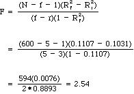
### Assumes that previous analyses are already run.

> anova(model2, model3)
______________________________________________________________

Analysis of Variance Table

Model 1: Optim ~ RelInf + RelInv + RelHope
Model 2: Optim ~ dummy1 + dummy2 + RelInf + RelInv + RelHope

  Res.Df  RSS Df Sum of Sq    F Pr(>F)
1    596 5520
2    594 5473  2        47 2.55  0.079 .
---
This F is on 2 and 594 df and is not significant, suggesting that the differences in optimism among the three groups can be attributed to differences on these three variables. (Sethi and Seligman came to a different conclusion, but that presumably just means that I was not completely successful in replicating their data.)
This final result tells us something important, in that it helps to identify the source of differences in Optimism among the three religious categories. There are certainly other differences among those categories, but after controlling for Religiosity, the category differences themselves are not significant. One would be justified in asking, however, what it means to talk about difference among levels of fundamentalism once we control for Religiosity. Differences in religious practice, the influence of religion, and views of the future are so integral to differences in Fundamentalism that it may not be meaningful to speak in such terms.
I have left a number of possible analyses undone for lack of space, but one point worth demonstrating involves plotting the relationship between Religiosity and Optimism. It is not possible to make a 4-dimensional plot involving three predictors and one criterion, but it is possible to plot the predicted values against the obtained values. What I am really plotting in that case is Optimism against an optimal linear combination of the three religiosity variables. I do this by applying the regression coefficients (including the constant) to each case, thereby generating predicted values for each subject, and then plotting predicted Optimism against obtained Optimism. Such a plot follows.
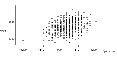
I present this plot simply to make a point about the significance of a correlation coefficient, whether that correlation be a simple correlation or a multiple correlation. In the discussion above we saw that the squared multiple correlation was 0.1031 and that it was significant at p = .0001. (It is what some people call "highly significant.") From this plot we can see that although the relationship is significant, there is a great deal of variability that the three religiosity variables do not predict.
This data set could be used to illustrate a number of different concepts that have not been mentioned here. For example, we could look at regression diagnostics. We could look at plots of individual variables, or at group comparison on all variables, not just optimism. In a complete analysis of these data we should do all of those and more. However for a classroom or textbook example, what we have done is sufficient. I will be happy to make the data available for those who wish to do more.
Aguinis, H. (1994). A QuickBASIC program for generating multivariate correlated random normal scores. Educational and Psychological Measurement, xx, xxx-xxx.
Kroll, M.D. (1994). A commentary on optimism, fundamentalism, and egoism. Psychology Science, 5, 56-57.
Sethi, S. & Seligman, M.E.P. (1993). Optimism and
fundamentalism. Psychological Science, 4, 256-259.
 Return to
Dave Howell's Statistical Home Page
Return to
Dave Howell's Statistical Home Page
Send mail to: David.Howell@uvm.edu)
Last revised 2/6/2018