Recent years have seen a large increase in the use of confidence intervals and effect size measures such as Cohen’s d in reporting experimental results. Such measures give us a far better understanding of our results than does a simple yes/no significance test. And a confidence interval will also serve as a significance test.
This document goes a step beyond either confidence intervals or effect sizes by discussing how we can place a confidence interval on an effect size. That is not quite as easy as it may sound, but it can be done with available software.
Almost nothing in this article is original with me. There are a number of sources that I could point to, but Busk and Serlin (1992), Steiger and Fouladi (1997), and Cumming and Finch (2002) are good sources. When it comes to actually setting confidence limits on effect sizes we need to use the non-central t distribution, and the explanation of that becomes tricky. I hope that my presentation will be the clear for everyone, but if it doesn’t work for you, go to the above references, each of which describes the approach in different terms.
What follows in this section should not be new to anyone, but I present it as a transition to material that will be new. I’ll begin with an example that will be familiar to anyone who has used either of my books. It concerns the moon illusion.
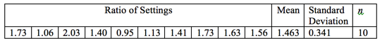
Everyone knows that the moon appears much larger when it is near the horizon than when it is overhead. Kaufman and Rock (1962) asked subjects to adjust the size of an artificial moon seen at its zenith to match the size of an artificial moon seen on the horizon. If the apparatus was not effective, there would be no apparent illusion and the ratio of the two sizes should be about 1.00. On the other hand, if there is an illusion, the physical size of the setting for the zenith moon might be, for example, 50% larger than the physical size of that moon seen on the horizon, for a ratio of 1.50. Kaufman and Rock collected the following data and wanted to set a 95% confidence interval on the size of the moon illusion.
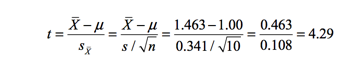
We will begin with our one sample t test on the sample mean. Normally we test a null hypothesis that the population mean is 0.00, but here if there is no illusion we would expect a ratio of 1.00, so our null hypothesis is μ = 1.00. Our t test is
The critical value of t at α = .05 on 9 df = +2.263, so we will reject the null hypothesis.
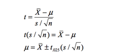
To calculate a confidence interval on μ we want to find those (upper and lower) values of μ for which our significance test is just barely significant. (In other words, we want to say something like “Even if true population mean μ were really as high as 3.2, we wouldn’t quite reject the null hypothesis that μ = 1.00.”) In this situation it turns out to be easy to create these limits because we can “pivot” the equation for t to give us a confidence interval on μ. We want to solve for those values of μ that would give us a t of exactly +2.263.
Notice that we have converted a formula for t into a formula for μ. I added the + in front of the t because I want both the upper and lower limits on μ. I also replaced “t” with t.025, 9 because I want the critical value of t on 9 df. This leads me to
Our confidence limits on the population mean of the moon illusion are 1.219 and 1.707. 95% of the time intervals computed by adding and subtracting the critical value of t times the standard error of the mean to the sample mean will encompass the true population mean. It is not quite correct to say that the probability is .95 that the true value of ?μ lies between 1.219 and 1.707, although you often find it stated that way. As others have said, our confidence is not in the numbers themselves but in the method by which they were computed.
In this particular case we are probably perfectly happy to say that the data show that the mean apparent size of the horizon moon is approximately 50% larger than the zenith moon. That is what a ratio of 1.50 means. But we have a somewhat unusual case where the numbers we calculate actually have some good intuitive meaning to us. But suppose that the 1.50 represented a score on a psychometric test. We would know that 1.5 is larger than 1.00, but that doesn’t give us a warm and cozy feeling that we have grasped what the difference means. (Remember that the 1.00 came from the fact that we would expect μ to be 1.00 if there were in fact no moon illusion.)
To come up with a more meaningful statistic in that situation we would be likely to compute an effect size, which simply represents the difference in terms of standard deviations. (In other words, we will “standardize” the mean.) We will call this statistic “d”, after Cohen. (A number of people developed effect size measures, most notably Cohen, Hedges, and Glass, and I am not going to fight over the name. Jacob Cohen was my idol, so I’ll give him the credit even though that may not be exactly correct. For a complete list see Kirk (2005) ). We could also fight over the symbol to be used (e.g., d, δ, Δ, g, ES, etc, but that doesn’t help anyone.) To calculate d in this situation we simply divide the difference between the obtained mean and our “null mean,” which is 1.00, by the standard deviation.
We will conclude that our result was about one and a third standard deviations above what we would expect without an illusion.
At this point you might want me to take the next step and compute a confidence interval around d = 1.36, but you’ll have to wait.
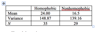
To take another example from at least one of my books, Adams, Wright, and Lohr (1996) ran an interesting study in which they showed sexually explicitly homosexual videotapes to people they had identified as homophobic or nonhomophobic. They actually expected the homophobic individuals to be more sexually aroused by the tape (for various psychoanalytic reasons), and that is what they found.
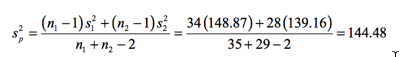
First we will pool the variances
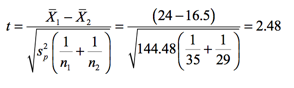
Then compute t
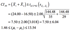
Now compute a confidence interval on the mean difference.
You will notice that although the difference is significant, the confidence interval on the difference is quite wide (approximately 12 units).
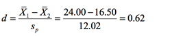
Now compute the effect size
We can conclude that difference between the two groups is about 2/3 of a standard deviation, which seems quite large.
There really should not be anything in what you have just seen that is especially new. We simply ran two t tests, constructed a set of bounds on the mean or the difference of means, and computed two effect sizes. I went through this because it leads nicely into confidence limits on effect sizes.
In the previous examples things were simple. We were able to go from a t test to a confidence interval by inverting the t test. (That is just a classier way of saying “turning the t test on its head.”) We went from solving for t to solving for μ with simple algebra that you probably learned in junior high. The reason that we could get away with that is that we were using a “central t distribution,” which is symmetrically distributed around 0. One limit would give you a t of 2.263 and the other limit would give you a t of -2.263. But when we come to effect sizes we need to use a noncentral t, which is a plan old t distribution that is not distributed around 0.00 and is not symmetric.
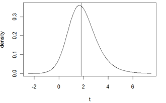
The figure below shows a noncentral t distribution on 9 df with a noncentrality parameter of 1.8. You can see that it is clearly non-normal. It is positively skewed. But what is a noncentrality parameter and why do we care?
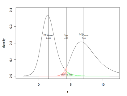
Think about the standard t test as a hypothesis test. We have
This formula is handy because if μ is equal to μ0 we are subtracting the true population mean from the sample mean and this is a central t distribution. And when we run a hypothesis test, we are asking about what the value would be if the null is true—if μ is equal to μ0. From here we can ask what values μ could take on and still not have the obtained t exceed the critical value (2.263 in our first example).
But a noncentral t is somewhat different. This is a t that is not distributed around 0, but around some other point. And that “other point” is called the noncentrality parameter (ncp). Suppose that we rewrite the above formula as:
If you clear parentheses and cancel, this is the same formula that we started with. In other words the first part of this formula is a central t but that bit on the end
moves the distribution left or right. That is the noncentrality parameter, and it is a standardized difference between the true mean and the mean under the null hypothesis. If μ = μ0 then the noncentrality parameter is equal to 0 and we are back to a central t distribution.
But why worry about the noncentral t distribution? One reason is that if we can put confidence limits on the noncentrality parameter itself, we can then, by a minor bit of algebra, turn those limits into confidence limits on effect sizes, because effect sizes are a linear function of the noncentrality parameter.
That doesn’t seem to help because now you will just change your question to “how will we put confidence limits on the noncentrality parameter.” But that is easy in principle, though not very easy if you don’t have a computer.
If we go back to our moon illusiion example, we found a t value of 4.29. If you had a program, like the one that generated the figure above, you could keep plugging in different possible noncentrality parameters until you happened to get one that had a cutoff of 4.29 for the lower 2.5%.
If you had a program called R, which is free, you could enter a command like pt(4.29, 9, ncp) and keep changing ncp until you got the answer you want. Look at the following sequence of output.
> pt(q = 4.29, df = 9, ncp = 5)
[1] 0.2758338
> pt(q = 4.29, df = 9, ncp = 6)
[1] 0.09950282
> pt(q = 4.29, df = 9, ncp = 6.9)
[1] 0.02908984
> pt(q = 4.29, df = 9, ncp = 6.95)
[1] 0.02692960
> pt(q = 4.29, df = 9, ncp = 6.99)
[1] 0.02530044
> pt(q = 4.29, df = 9, ncp = 7.00)
[1] 0.02490646
> pt(q = 4.29, df = 9, ncp = 7.01)
[1] 0.0245177
The lines that begin with the “>” are the commands. The first one says “what is the lower tailed probability of getting t = 4.29 on 9 df when ncp = 5. (R uses the label “q” for what we call “t.”) The probability was 0.2758. Well, that didn’t work because we wanted .025, so I increased ncp and moved somewhat closer to 0.025. I kept increasing ncp, moving closer, until I overshot. It looks like my best guess was ncp = 7.00.
Then I tried working on the other end. I want an ncp that will have a probability of .975 of getting a t of 4.29 or below. I get the following sequence, again starting off with any old guess. (If you enter the parameters in the correct order you don’t have to label them as “q =”, etc.)
> pt(4.29, 9, 1.5)
[1] 0.973518
> pt(4.29, 9, 1.45)
[1] 0.9757474
> pt(4.29, 9, 1.44)
[1] 0.9761741
> pt(4.29, 9, 1.46)
[1] 0.9753144
> pt(4.29, 9, 1.47)
[1] 0.974875
> pt(4.29, 9, 1.465)
[1] 0.9750955
So now I know that the 95% confidence interval on the noncentrality parameter is P(1.465 < ncp < 7.00) = .95.
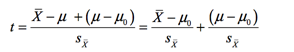
The following graph plots the two noncentral t distribution, each of which cuts off 2.5% in the tail at tobt = 4.29. You can see that the distributions differ in shape. The corresponding noncentrality parameters are shown by vertical lines.
Now we can find the 95% confidence interval on d*. (I use d* to indicate the true parametric value of the effect size. I could use a Greek letter, but that gets messy later.) I can show, but won’t, that
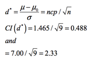
So the confidence interval on d* is 0.488 < d* < 2.33.
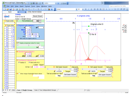
Many readers are probably not familiar with R. Well, Cumming and Finch (2001) have something for you! They have written a script that runs in Excel that will do the calculations for you—and a lot faster than I did them. It is called ESCI, and you can download it at http://www.psy.latrobe.edu.au/esci . They charge a small amount (I think that I paid $15) but they have a trial version that you can play with for free. It takes a bit of playing to get used to it (Don’t be afraid to click on things to see what happens.), but it is worth it. Their output is shown below. You will see that their limits are not quite the same as mine (their CI was 0.466 – 2.216), but they came up with different ncp values, which just means that they solved a messy computer coding problem by a different algorithm. (They use Δ for the ncp and δ for d*.)
From the two-sample example we have
t = 2.48, df = 62, d = 0.62
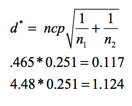
Playing around to find the ncp for which t = 2.48 is at the lower or upper .025 level, I find that the limits on ncp are 0.465 and 4.48.
This time the relationship between the CI on ncp and the CI on effect size is
That result agrees nicely with Cumming and Finch.
I am not going to work through other effect size limits here, but there is good coverage in the paper by Steiger and Foulardi. They cover ANOVA, R2, analysis of covariance, and put confidence limits on power estimates.
What I have given you in this document is a way of computing confidence limits on a single effect size. In other words, you go out and conduct a study with ni subjects in each condition, compute an effect size, and then compute a confidence limit. That’s just fine. But suppose that you ran some single-subject studies on 4 people. (You collect behavioral data on one subject before an intervention, then intervene, and then collect more behavioral data after the intervention. And you repeat this process for 3 other subjects, but keeping the data separate for each subject.) For each subject you could calculate an effect size. With suitable assumptions you could calculate confidence limits on that effect size using the noncentral t. But you could also pull together the effect sizes for each subject and use those to calculate confidence limits on an overall effect size by using the same methods that we used above to calculate confidence limits on the mean. I hope to write this up soon.
dch:
David C. Howell
University of Vermont
David.Howell@uvm.edu