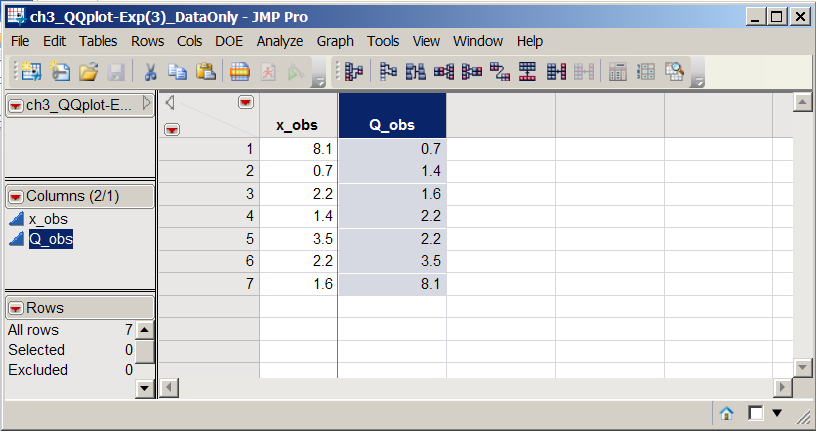
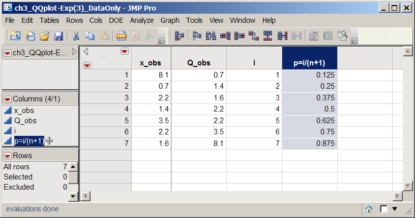
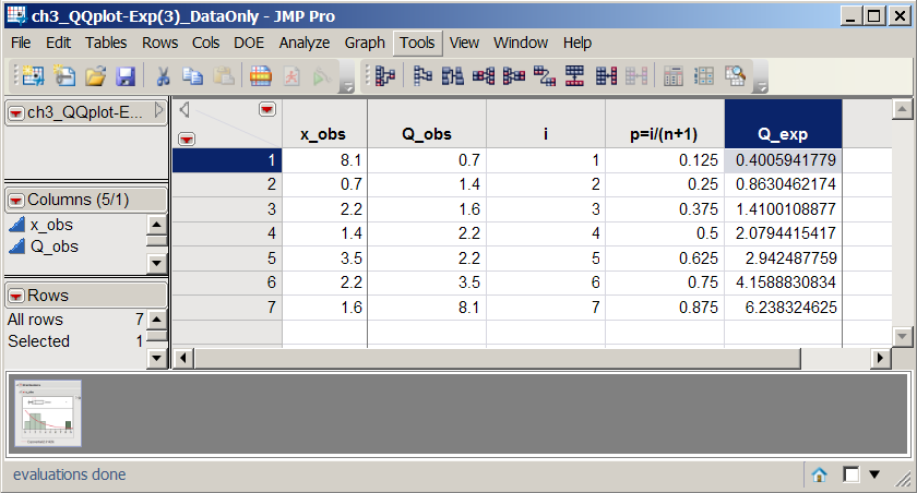
Seven values were observed for interarrival times at a checkout counter in a busy store. It is believed that an exponential distribution with parameter 3 might model the observed data well.
The observed values for X are in Column 1 and the corresponding oberved quantiles (Q_obs) are in Column 2. These are the sorted values for x_obs.
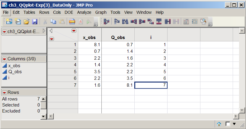
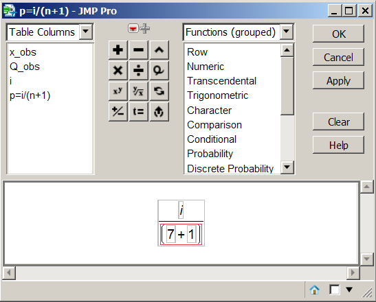
Rename Column 3 as "i" with the observation numbers and Column 4 as "p=i/(n+1)"
Right click on the top cell of Column 4 and select "Formula" (or you can click the top cell to highlight the column and select "Formula" from the "Cols" menu). Select "i" from the left column "division" from the keypad and then 7+1 in the denominator, then click "ok".
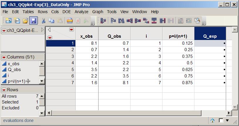
Rename Column 5 as "Q_exp" for the expected quantiles, which come from the inverse CDF evaluated at p [i.e., ln(1-p)*(-3)].
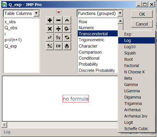
Right click on the top cell to enter a Formula and select "Transcendental" and "Log".
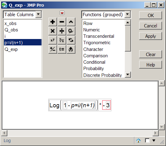
Enter (1-p) * -3 [use the "-", "*", and "+/-" (for the -3) from the keypad to enter arithmetic operators].
NOTE: use the up & down arrow keys to move the red rectangle indicating the "scope" in the formula.
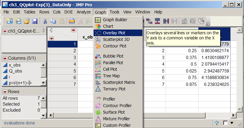
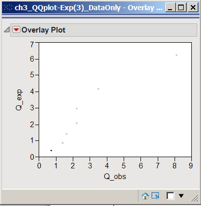
Click the Graph menu and select Overlay Plot
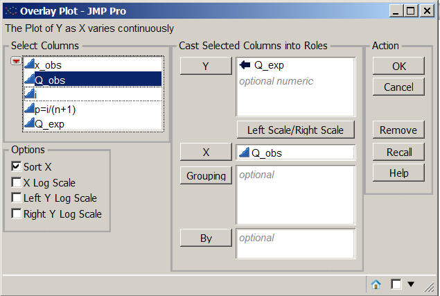
Select Q_exp as the "Y" variable and Q_obs as the "X" variable.
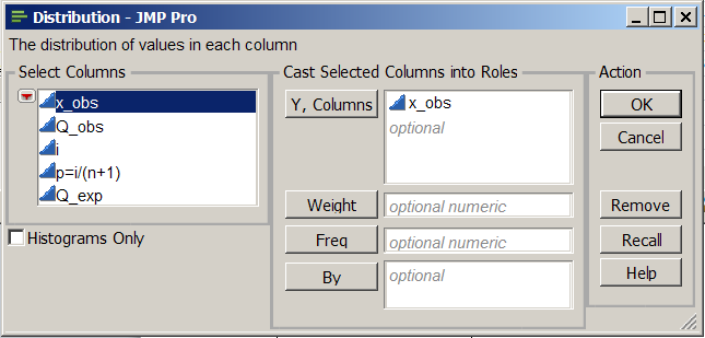
To use JMP's built-in features, click the Analyze menu and select Distribution
and then select x_obs as the "Y,Column" variable.
Click on the red triangle next to x_obs and select "Continuous Fit" and "Exponential"
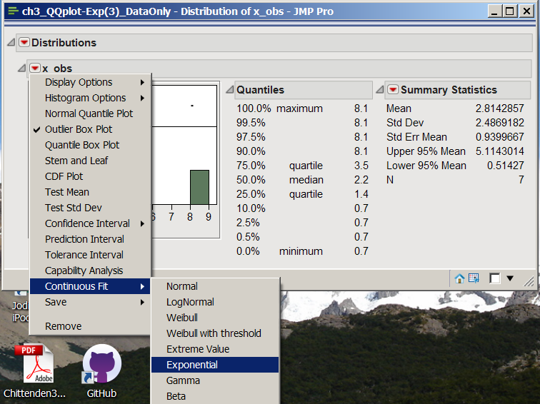
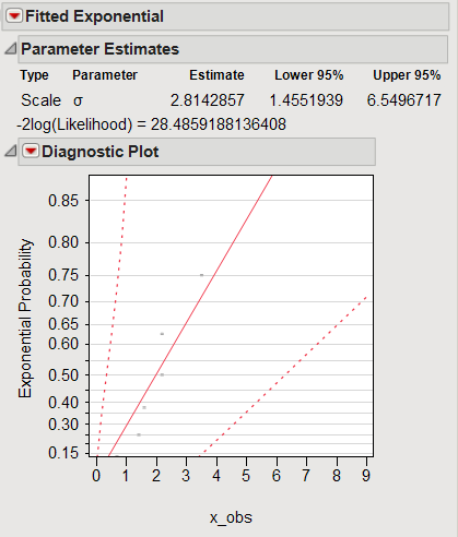
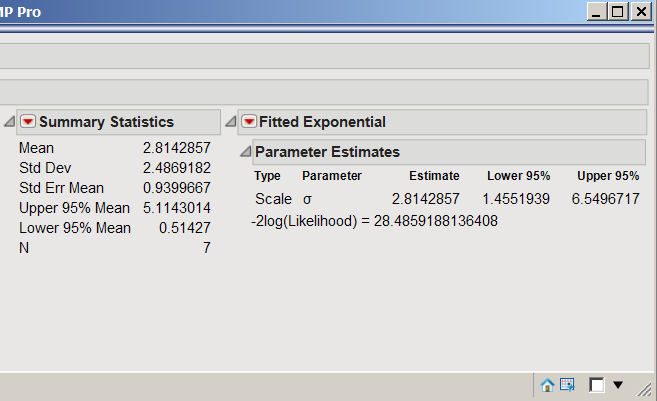
This gives the estimated parameter of the "best" exponential RV to model these data (2.814 here, which is the mean).
Click on the red triangle next to Fitted Exponential and select "Diagnostic Plot"
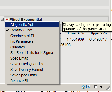
This gives a Q-Q plot based on the "best-fit" exponential model.