The modeling type for x was changed to ordinal by clicking on the blue triangle and selecting ordinal. This gives a green histogram icon.
Rutherford and Geiger (1910) observed the collisions of alpha particles emitted from a small bar of polonium with a small screen placed at a short distance from the bar. The number of such collisions in each of 2608 eight-minute intervals was recorded; the distance between the bar and screen was gradually decreased so as to compensate for the decay of the radioactive substance. A Poisson distribution with lambda = 3.87 was fitted to the data. [Rutherford, Chadwick, and Ellis (1930)]
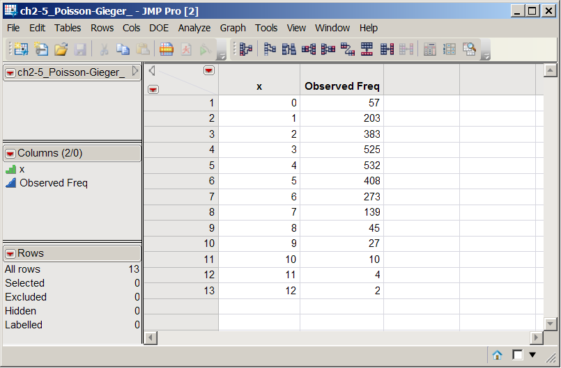
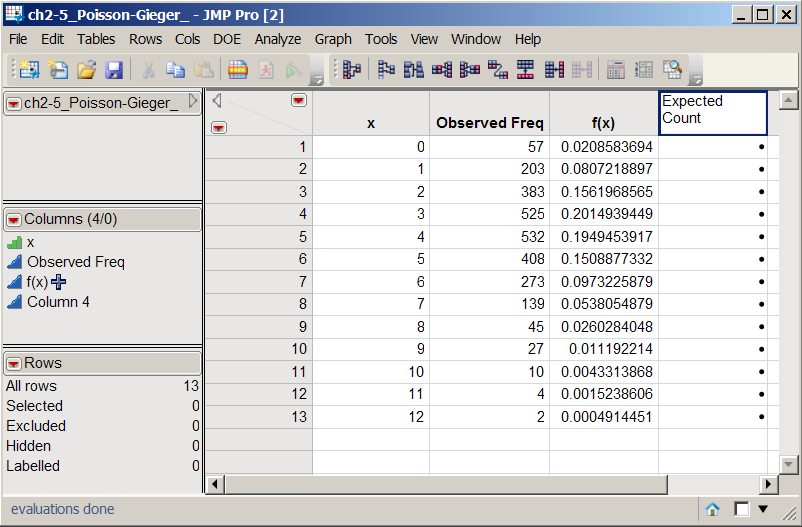
The observed values for X are in Column 1 and the observed frequencies in each interval are in Column 2.
The default modeling type is continuous (blue triangle next to Observed Freq) since numerical data was entered.
The modeling type for x was changed to ordinal by clicking on the blue triangle and selecting ordinal. This gives a green histogram icon.
Double click on the third column to create a new variable.
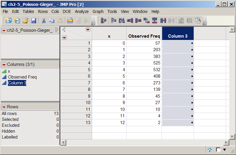
This column will hold the PMF, f(x).
Right click on the top cell of f(x) and select "Formula" (or you can click the top cell to highlight the column and select "Formula" from the "Cols" menu).
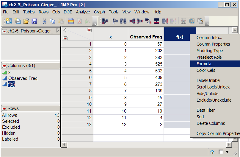
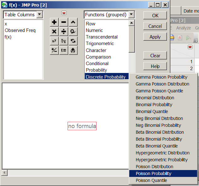
Under "Discrete Probability", select "Poisson Probability".
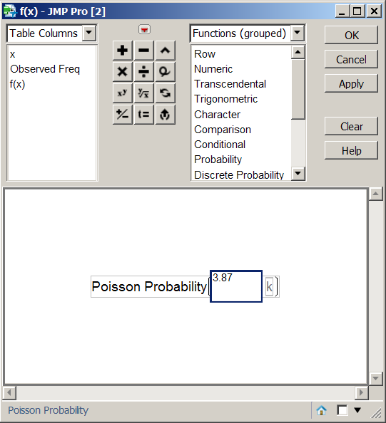
Enter a value for lambda (3.87 here).
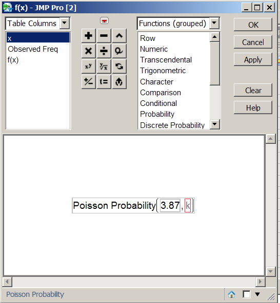
Click on "k" outlined in the red box, and select "x" from the table columns and click OK.
This sets the values at which to evaluate the Poisson PMF.
This gives the Poisson probabilities.

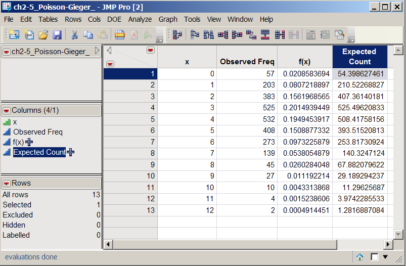
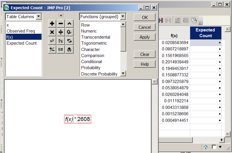
Double click on the fourth column to create the expected counts.
The formula for the expected counts is the number of trials [n] times the probability of a x successes [f(x)].
Since the Poisson approximation is good, the expected counts are pretty close to the observed counts.