Soil Carbon and Other Quality Indicators
in Managed Northern Forests
Home

Methods

Summary of Results

Contact Us

Research Sites:
ATLAS Land
Coolidge SF
Emerald Lake SP
Green Mountain NF
Groton SF
Hinesburg TF
Jericho RF (JRF)    
Marsh-Billings-Rockefeller NP

Starksboro TF
Steam Mill Brook WMA
Sterling TF
The Waterworks Property
Willoughby SF


Plot Design

The plot design and vegetation description methods used in this study follow the Forest Inventory and Analysis (FIA) protocol, to allow for comparisons.

One plot consisted of:
  • six soil subplots at 90 feet from the center of the plot, every 60 degrees (three additional subplots than the FIA protocol, depicted on the image on the right). Pits were only sampled at soil subplots 1, 3, and 5. Cores were sampled at each soil subplots.
  • four vegetation subplots, one at the center of the plot, the three others every 120 degrees (grey circles on the image). Each vegetation subplots has a radius of 24 feet.

The GPS coordinates of the center of each plot were recorded using a high-precision GPS.

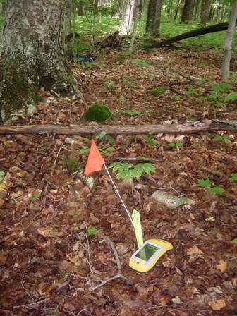
A yellow stake was pounded in the ground at the center of the plot as permanent marker.
Permanent Marker and GPS at Center of Plot

   Plot Design  |  Measuring Soil Carbon |  Calculating Soil Carbon
Measuring Above Ground Carbon  |  Calculating Above Ground Carbon
Home

Methods

Summary of Results

Contact Us

Research Sites:
ATLAS Land
Coolidge SF
Emerald Lake SP
Green Mountain NF
Groton SF
Hinesburg TF
Jericho RF (JRF)    
Marsh-Billings-Rockefeller NP

Starksboro TF
Steam Mill Brook WMA
Sterling TF
The Waterworks Property
Willoughby SF

Measuring Soil Carbon

In this study, three 40 x 60 cm soil pits were excavated at each site, down to a depth of 40-inch, bedrock, or water.


Soil Pit
Soil horizons can be identified after excavating a soil pit. Horizon descriptions can be used to assign a soil series to each soil described ("soil series" is the soil science equivalent of  the term "species" used in biology).

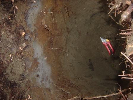
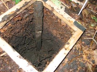
Soil horizons can be differentiated through a change in color or texture, a change in the abundance of roots, the presence or absence of redoxomorphic features, etc. For example in the picture on the right, an E horizon (grey color) and a Bs horizon (reddish color), can very easily be identified.

The amount of carbon can vary strikingly between horizons and it is therefore necessary to sample soils by horizons when quantifying soil carbon. Soil samples were collected from each soil horizon and analyzed in the lab.


Soil Horizons
The forest floor, also known in soil science as the organic soil horizons (Oi, Oe, and Oa in the US taxonomic system), was collected by cutting three 15 x 15 cm squares in the forest floor, at each of the six soil subplots.

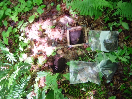
Organic soil samples were analyzed in the lab. As the forest floor was collected over a known area, carbon per hectare (or acre) can easily be quantified.

Sampling Organic Horizona
Soil samples were collected from three soil pits. In order to translate from percent carbon by weight to carbon per hectare (or acre), soil bulk density needs to be know.

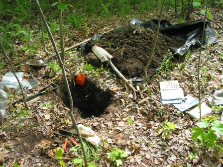
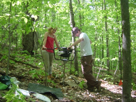
To measure and calculate bulk density, we used a power auger equipped with a diamond-tipped core. We then collected cores of known depth (usually 10-20 cm) at each of the 6 soil subplots.

Cores were collected down to bedrock, water, or 100 cm depth, whichever came first. Soil samples obtained from cores were also analyzed in the lab.


Pace Goodman and Chauncey Smith augering
The power auger  also allowed us to estimate soil stoniness. Stoniness is important because the quantity of rocks in the soil affects the calculation of carbon per hectare (or acre).

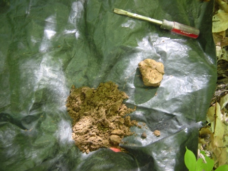
The picture on the right illustrates how the power auger cored through a rock, allowing us to collect both the rock and soil sample.


Soil and Rock from Core
Calculating Soil Carbon
  • Bulk density was calculated for each mineral soil horizon using data obtained from cores sampled next to the soil pits:
(bulk density) = [(soil core weight, oven dry) - (root weight) - (rock weight)] / [(core volume) - (rock volume)]
  • Percent carbon and nitrogen by soil dry weight were measured on a Thermo Scientific Flash EA 1112 Nitrogen and Carbon Analyzer for Soils, Sediments and Filters
  • Carbon Pool in Mineral Soil (Mg/ha):
(C in Mineral Soil) = (bulk density) x (horizon depth) x (percent carbon)
  • Carbon Pool in Organic Soil (Mg/ha):
(C in Organic Soil) = {[(soil weight, oven dry) - (root weight) - (twig weight) - (rock weight)] / (area sampled)} x (percent carbon)


Home

Methods

Summary of Results

Contact Us

Research Sites:
ATLAS Land
Coolidge SF
Emerald Lake SP
Green Mountain NF
Groton SF
Hinesburg TF
Jericho RF (JRF)    
Marsh-Billings-Rockefeller NP

Starksboro TF
Steam Mill Brook WMA
Sterling TF
The Waterworks Property
Willoughby SF


Home Page  |    Plot Design  |  Measuring Soil Carbon |  Calculating Soil Carbon
Measuring Above Ground Carbon  |  Calculating Above Ground Carbon
Measuring Above-Ground Carbon
In order to calculate carbon stored in the aboveground biomass, we measured tree diameter (DBH) and height  (for trees >2 inches) in each of the four vegetation subplots.  Trees were also identified by species.

Each vegetation subplot contained a microplot where the percent ground cover occupied by moss, lichen, shrubs, etc. was estimated.

Saplings and seedlings
were counted in each microplot.

To estimate the quantity of carbon stored in down woody material, we measured down trees and branches following the FIA protocol.


Emily West measuring trees
Calculating Above-Ground Carbon
  • Above-ground biomass (live trees):
bm = Exp(B0+B1 ln(DBH))

bm = total aboveground biomass (kg dry mass)
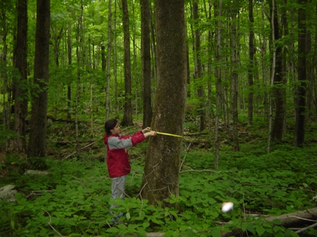
DBH = diameter at breast height (cm)
Exp = exponential function
ln = log base e
For more details, see: Jenkins J.C., Chojnacky D.C., Heath L.S., and Birdsey R.A., National-Scale Biomass Estimators for United States Tree Species, Forest Science, Vol 49, No.1, February 2003
  • Carbon stored in above-ground live trees:
Estimated to be 50% of above-ground biomass in live trees.
  • Down Woody Material, dead standing trees, and ground cover: coming soon
  Plot Design  |  Measuring Soil Carbon |  Calculating Soil Carbon
Measuring Above Ground Carbon  |  Calculating Above Ground Carbon

Home Page   |   Contact Us   |   Summary of Results   |   Methods
ATLAS Land  |  Coolidge SF  |   Emerald Lake SP  |  Green Mountain NF  |  Groton SF  |  Hinesburg TF  
Jericho RF  |   Marsh-Billings-Rockefeller NP  |  Starksboro TF  |  Steam Mill Brook WMA 
Sterling TF  |  The Waterworks Property  | 
Willoughby SF