Lab 2
Summarizing land
cover and LiDAR surfaces by parcel at a fine scale
Due
Feb. 1
- Again map a drive to \\zoofiles\gradgis. Open Arc Catalog and in it copy the entire Randalstown directory from within NR245 directory. This lab will involve large datasets so I recommend that you copy the data to the temp drive and do your work from there. At the end of the lab, copy the entire directory from the temp directory back to your Zoo account.
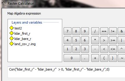
- First
we will summarize building heights by building, just to get an idea of how
LiDAR data works. The intuitive thing to do is
subtract the lidar_bare_r layer from the lidar_first_r layer using raster map algebra. However,
there are tiny errors in the data that will result in a bunch of
artificial “pits” or pixels with values less than zero. To deal with this
we’ll use the raster “conditional” function to essentially set any
resulting pixels that would have been less than zero to zero. Con uses the
following syntax: CON(if statement, then do
statement, else do statement). To access it, open Arc Toolbox and click on
Spatial Analyst Tools>>Map Algebra>>Raster Calculator. Make
sure to specify the output path to your working directory and call it lidar_diff_r. Your CON function should like something
like this:
- We’ll use this new layer to estimate building height. Load up the buildings_R layer from the Randalstown geodatabase and then use zonal statistics to summarize height by building. However, just like with last lab, you’ll need to create a join field, so open the attribute table, create a new field called “join1” and use the field calculator to set it equal to ObjectID. In toolbox click Spatial Analyst Tools>>Zonal>Zonal statistics as table. Make buildings_R as zone dataset, join1 as the zone field, and choose lidar_diff_r as the value raster. Save the output in your Randalstown folder and call it “bldg.” Open the attribute table for buildings_R and create a new integer field called “height.” Then do a tabular join to join the resulting table to buildings_R. Use the field calculator to set it equal to “bldg.MAX.” Now you can remove joins on that layer. NOTE THAT IF IN THIS ZONAL STATISTICS FUNCTION OR ANY IN THE FUTURE THE TOOL DOES NOT SUCCESSFULLY EXECUTE, JUST GO TO FILE>>NEW AND RE-ADD THE TWO LAYERS YOU NEED FOR THE ZONAL STATISTICS. IT SHOULD WORK THEN
- Now open Arc Scene and load up buildings_R, Land_Cov_R, and lidar_bare_r. Double click on the Land_Cov_R item in the TOC and go to the base heights tab. Click on the radio button that says ”floating on a custom surface”and choose “lidar_bare_r”. Then go to the rendering tab and check “shade areal features”. The click OK. Then click View>>properties and select a vertical exaggeration of 2. Go to the Illumination tab and change sun altitude to 40 degrees and contrast to 60. Click OK. Now double click on buildings_r in the TOC and under “base heights” click the radio button for “”floating on a custom surface” choosing lidar_bare_R (which it probably already has listed in the text box). Then click the extrusion tab and check the “extrude features in layer check box”. In the Extrusion value window below, click the calculator icon to the right and click on “height.” Under rendering tab check the “shade areal features” box.” In symbology, choose a color that contrasts with the background. Click OK. take a screencapture of what you see in 3D perspective. Note that lidar_bare_r is never checked in the Table of Contents.
- Now we
will estimate the height of the tree canopy. First we’ll create a raster
layer giving the height of trees only. This time we’ll use a command call SetNull that does something similar to CON, but
specifically when you want to return a null value for some of the pixels.
In this case we want to set all pixels without a Land cover code of 2
(trees) to null, so they don’t appear at all. Open the raster calculator and
write SetNull([land_cov_r] <> 2, [lidar_diff_r]).
Note that <> means “not equal to.” What this means is, if land cover
is not type 2 (trees), then the pixel value is set to null, otherwise to lidar_diff. Call the output Lidar_trees_r.
Make a hillshade of the Lidar_tree_r
layer in spatial analyst and in the TOC, move the hillshade
right below the trees layer. Set the symbology
of the lidar_tree_r layer to green graduated
color and transparency (under display tab) to 25%. Now, the trees should
like nice and textured. Display the
textured trees overlaid on parcels and buildings and screencapture
the result.
- Now summarize tree cover percentage and height by parcel. Let’s start by making a raster 1/0 layer showing tree pixels only. In raster calculator type [land_cov_R] == 2. You won’t need this any more after this so you don’t have to make this calculation layer permanent. But you will use it now for zonal statistics. Name the raster calculator output "tree." Then gGo to spatial analyst>>zonal statistics and choose parcels_R as the zone dataset join1 as the zone field, tree as the value raster, check the “join output table box”, uncheck the chart box, and save the output table in your Randalstown folder as tree. Join the resulting table to the parcels_R layer. Open the attribute table for the parcel layer from the TOC then, create a new field set to Double called P_tree . Right click on the P_tree field heading and click the field calculator. Set the new field equal to “tree.MEAN.” Then right click and hit joins>>remove all joins. Next we’ll summarize the tree height by parcel. Again use zonal statistics, only this time choose “lidar_trees_r” as the input raster. Call the output table treeht.dbf. Make two new fields (set to double), one called mean_ht and one called max_ht. Use the field calculator and…you guessed it…calculate the mean_ht field to be equal to treeht.MEAN and the max_ht field to be equal to treeht.MAX. Again, remove all joins. Remove the temporary “trees” 1/0 layer.
- Now
let’s calculate some variables that we think might help explain variation
in tree height. First we’ll summarize distance to water, an obvious
predictor. Go ahead and load up NR245\lab_data\NHD_Lines_GF in your view (if it’s slow to load, copy
it to your geodatabase). Also load up the BG_R
layer into your view. Now we’ll
create a straight line distance raster layer for the Randalstown
area. In toolbox go to Spatial Analyst>>distance>>Euclidean
Distance. Choose NHD_lines_GF as the distance to
layer and choose an output cell size of 3 meters. Click “environments and
click on “processing extent”, setting it equal to BG_R, then go to “raster
Analysis” and set Mask to BG_R too. You can save the output as a temporary
file. Then do zonal statistics (spatial analyst>>zonal statistics)
and set Parcels_R as the zone dataset, ACCTID2
as the zone field, Distance to NHD lines (or whatever you called your
straight line distance raster layer) as the value raster. Call the output
table wat.dbf. Click ok and then join tables and
open the attribute table for parcels_R. Add a
new field (long integer) called D2wat. Use the field calculator to set
that new field equal to the “wat.Mean” field.
Then remove the joins for that layer (right click on the
layer>>joins>>remove). Make
a graduated color map of parcels where the color represents the distance
to water and take a screencapture.
- Now we’ll add another variable. We imagine that properties that are located near empty lots (which tend to be forested in this suburb—at least one of these empty lots is a large park) will have bigger trees. Go to select by attribute for Parcels_R and type [bldg_type] = '999' OR [bldg_type] Is Null. This selects all parcels with no dwelling. Export this to a new feature class in your geodatabase called no_dwel. Now we want to delete all these records from our Parcel_R layer. Without clearing the selection, now go into edit mode (activate the Editor toolbar and click Editor>start editing, making sure that Parcels_R is listed as the target) and delete your selection by simply clicking the delete button. If it doesn’t delete, then try redoing the attribute query in edit mode and then hitting delete. Then click Editor>>stop editing and save your edits. Get rid of the raster distance to water layer from your view. Now let’s figure out how far each parcel is from an empty lot. Again we’ll use straight line distance and zonal stats. This time use spatial analyst to generate a layer giving straight line distance to the nearest empty parcel with pixel size set to 3 meters and the same environment settings used for the distance function earlier. After generating this, then do zonal statistics again, just like the last time, except your input raster will be the layer you just created. Call the output table something like nodwel.dbf. Again, create a new field in parcels_R, this time called D2nodwel and set it to integer. Then, use the field calculator to set that new field equal to nodwel.MEAN. Remove joins again.
- Now close Arc Map and open SPlus. To import data from a Geodatabase go to file>>import data>>from database. Under data source choose MS Access Database and a browser window will come up. Browse to your Randalstown geodatabase (it must be a personal geodatabase, not a file geodatabase, for this to work) and then choose parcels_R under Table name. Keep everything else as it is and click OK. You should now have a data table with the attributes. Let’s add one more attribute: housing age (right now year built is stored as a year). Open the table, scroll to the first empty column and right click in the heading. Click insert column. Under the name put Yearsold and under fill expression put 2005-YearBuilt. Now let’s run some regressions. Go to statistics>>regression>>linear. Let’s start with a univariate regression looking at the relationship between house age and tree cover. Let’s regress percent tree cover (P.tree) against years old. To do this click on P.Tree under “dependent variable” and Yearsold under “independent.” You can manually manipulate the formula where it says “formula.” Then, click Apply. Look at the results. Q1. What is the coefficient and P value on Yearsold? Is this coefficient statistically significant, and how do you know? According to the coefficient, how much does percent tree canopy increase with each additional decade of housing age? (keep in mind that P_tree is stored as a decimanl-e.g. 0.1 means 10%). Now, for comparison, try regressing max.ht (dependent) against Yearsold (independent). Q2. Report the coefficient and P value. This model should have a lower R-squared than the previous one. Explain what that tells you.
- Next, let’s do a multivariate regression. Let’s look at the relationship between max tree height and the following independent variables: yrsold, d2nodwel, d2wat, lot size, assd.land (assessed land value) and price. Q3. Report which of the variables are significant and which are not? How do you know this? Which significant variables are associated with greater tree height and which with lower tree height? Interpret the coefficient on d2water: what happens to tree height as you move away from water? Drop the insignificant variable(s) in your model interface, but this time we’ll do a diagnostic: click on the “plot” tab, and check the residuals vs. fit and Residuals Normal QQ plots. Look at the residual vs fit plot and notice how there are no major patterns in residuals, but rather a very random spread, which is a good sign. Note from the QQ plot that there are slight deviations from normality, but not too bad.
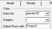
- Now
try adding another independent variable this will totally change this
model. The term is P.tree, but before running
the model we are going to specify that we only want to run this on a
subset of the data—that is parcels where percent tree cover is greater
than zero. To do this, in the “Subset rows with” type P.tree>0
 . This time include plots for “Residuals
vs. fit”. Run the model. Q4. Describe what happens to model fit
and which variable now becomes insignificant. Take a screencapture
of the Residuals vs. fit plot. You should see more of a pattern in
this plot than in the previous model, indicating that a transformation or
higher order term is necessary. Now
let’s try transforming the P.tree variable. In
the model interface, drop the insignificant term and replace P.tree with “log(P.tree).” Now rerun the model and again screencapture the residuals vs. fit plot. Q5
Describe the change in model fit and what the change in the residual plot
suggests.
. This time include plots for “Residuals
vs. fit”. Run the model. Q4. Describe what happens to model fit
and which variable now becomes insignificant. Take a screencapture
of the Residuals vs. fit plot. You should see more of a pattern in
this plot than in the previous model, indicating that a transformation or
higher order term is necessary. Now
let’s try transforming the P.tree variable. In
the model interface, drop the insignificant term and replace P.tree with “log(P.tree).” Now rerun the model and again screencapture the residuals vs. fit plot. Q5
Describe the change in model fit and what the change in the residual plot
suggests. - Finish up by combining your screencaptures and answers together in a document, turn it into a PDF and upload.