Standard Error Bars in Excel
Enter the data into the spreadsheet. Under the columns of data calculate
the standard error of the mean (standard deviation divided by the square root
of the sample size), and calculate the mean. The spreadsheet with the
completed graph should look something like:
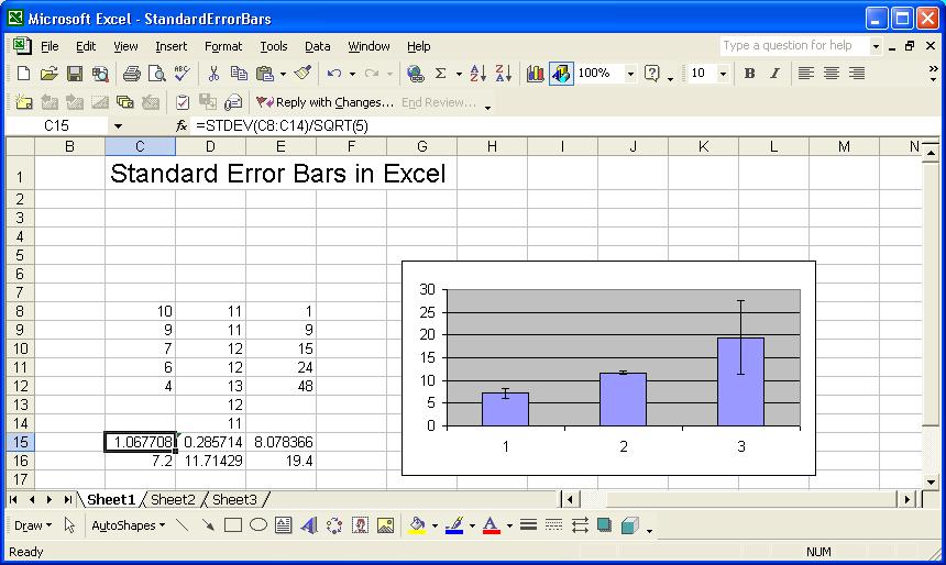
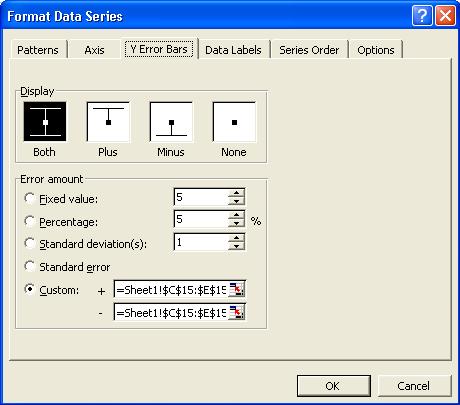
Create your bar chart using the means as the bar heights. Then, right
click on any of the bars and choose Format Data Series. Click
on the Y-Error Bars tab, Choose to display Both error bars,
and enter the ranges for standard errors (cells C15:E15 in the example
above) in the Custom Error amount. Be sure to both add and subtract
the standard errors (C15:E15 ) in the custom amount. The dialog
box should look like:
Click OK and the graph should be complete. Be sure to add a title,
data source, and label the axes.